Methodological annex
Updated 23 June 2022

© Crown copyright 2022
This publication is licensed under the terms of the Open Government Licence v3.0 except where otherwise stated. To view this licence, visit nationalarchives.gov.uk/doc/open-government-licence/version/3 or write to the Information Policy Team, The National Archives, Kew, London TW9 4DU, or email: psi@nationalarchives.gov.uk.
Where we have identified any third party copyright information you will need to obtain permission from the copyright holders concerned.
This publication is available at https://www.gov.uk/government/statistics/measuring-tax-gaps/methodological-annex
Chapter A: Introduction
Methodology
A1. This document provides further details of the data and methodology used to produce estimates of the tax gap published in Table 1.1 ‘Tax gap components 2020 to 2021 estimates’ of ‘Measuring tax gaps 2022 edition’.
A2. There are numerous methodological approaches to measuring tax gaps.
A3. Top-down methods use external independent data sources to estimate total consumption of taxable products to calculate the total theoretical liabilities; the tax gap is the difference between the total theoretical liabilities and the tax actually paid. An example of this is the Value Added Tax (VAT) gap.
A4. Bottom-up methods include a number of techniques:
-
random enquiry programmes – these are full enquiries opened by HMRC compliance officers into a randomly selected sample of taxpayers
-
statistical methods – unlike random enquiry programmes these use risk-based enquiries that are not representative of the whole population, and require statistical methods to scale up the results to the whole population
-
population surveys – we use results from a bespoke research survey to estimate part of the hidden economy tax gap
-
management information – these methods use management information such as:
- risk registers (a list of identified tax risks, together with information such as estimated value, nature and status)
- data extracted from accounting systems
- other databases or systems used to manage HMRC’s business
A5. The total tax gap is estimated using established statistical and experimental methods. Experimental methodologies are used to produce illustrative estimates where there are no direct measurement data. For these tax gap components, we use the best available data and simple models to build an illustrative estimate of the tax gap.
A6. We employ the most appropriate methodology for each tax gap component, based on the factors listed below:
-
availability of quality HMRC data
-
availability of quality independent data
-
structure of the tax regime
-
cost and impact for both HMRC and taxpayers
-
level of granularity demanded
A7. Generally, following good international practice, we use ‘top-down’ methodologies for indirect taxes and ‘bottom-up’ methodologies for direct taxes. The tax gap estimates may, however, also be produced by compiling the results from a combination of 2 or more methods.
Methods used to calculate the tax gap
A8. Table A.1 below shows the general methodological approach used to calculate each tax gap component.
Table A.1 Tax gap methodologies
| Top-down | Bottom-up (management information) | Bottom-up (statistical and survey) | Bottom-up (random enquiries) | Experimental |
|---|---|---|---|---|
| VAT all businesses | Hidden economy | PAYE mid-sized businesses | PAYE small businesses | Other excise |
| Alcohol duties | Alcohol duties | CT mid-sized businesses | CT small businesses | SA large partnerships |
| — | — | CT large businesses | SA business and non-business | PAYE large businesses |
| — | — | Inheritance Tax | Diesel duties | Avoidance |
| — | — | Hidden economy | — | Stamp taxes |
| — | — | — | — | Other remaining taxes |
| — | — | — | — | Tobacco duties |
Notes for Table A.1
-
Alcohol duty tax gaps are produced using both top-down and bottom-up methodologies.
-
Hidden economy tax gaps for ghosts and moonlighters are produced using bottom-up management information and bottom-up statistical and survey methodologies.
A9. Figure A.1 below shows a summary of the tax gap by methodology. A degree of assumption and judgement has been applied to attribute some elements of the tax gap to methodology types, especially where a combination of methods is used.
Figure A.1 Tax gap by methodology (£ billion)
| Methodology | Tax gap (£ billion) |
|---|---|
| Top-down | £9.45bn |
| Bottom-up (management information) | £1.02bn |
| Experimental | £6.79bn |
| Bottom-up (statistical and survey) | £4.09bn |
| Bottom-up (random enquiries) | £10.88bn |
A10. Over time, we have tried to estimate more of the tax gap using an established top-down or bottom-up methodology and rely less on experimental methods. This is difficult to show on a comparable basis as the tax gap for earlier years is often revised between editions either when methodological improvements are made or the underlying data are updated – and the overall value of the gap changes over time.
A11. Table A.2 sets out what proportion of the total tax gap was classed as established or experimental in the last 6 editions of ‘Measuring tax gaps’. This shows 79% of the tax gap was estimated using established methods in the 2022 edition of ‘Measuring tax gaps’ compared to 70% in the 2016 edition.
A12. The proportion of the tax gap based on established methodologies has decreased from 86% to 79% since MTG21. This is driven by changes in the tobacco tax gap classification.
A13. Due to significant changes in the underlying survey data, the tobacco tax gaps (cigarettes and hand-rolled tobacco) have been held constant as a percentage of total theoretical liabilities since 2017 to 2018. As this projection method has now been in place for 3 years, the methodology has been moved from established to experimental.
Table A.2 Total tax gap by established and experimental methodologies over time
| Measuring tax gaps edition | Experimental methodology | Established methodology |
|---|---|---|
| MTG 2016 | 30% | 70% |
| MTG 2017 | 24% | 76% |
| MTG 2018 | 24% | 76% |
| MTG 2019 | 24% | 76% |
| MTG 2020 | 15% | 85% |
| MTG 2021 | 14% | 86% |
| MTG 2022 | 21% | 79% |
Tax gap development programme
A14. As official statistics, our tax gap estimates are produced with the highest levels of quality assurance and adhere to the Code of Practice for Statistics framework. This code assures objectivity and integrity – providing the framework to ensure that statistics are trustworthy, good quality, and valuable. It also provides producers of official statistics with the detailed practices they must commit to when producing and releasing official statistics.
A15. In April 2020, the Office for Statistics Regulation (OSR) published a report, Strengthening the quality of HMRC’s official statistics, in which it recommended that HMRC takes action to enhance the quality of its official statistics. Also in 2020, the National Audit Office report, Tackling the tax gap and the Public Accounts Committee report, Tackling the tax gap made recommendations that HMRC reduce the level of tax gap estimate uncertainty and clearly explain the extent and nature of uncertainty in the tax gap publications.
A16. To support these recommendations, we are publishing a tax gap development programme. This contains:
-
a summary of the improvements to the estimates introduced in the current edition of ‘Measuring tax gaps’ publication
-
a high-level summary of development priorities to improve the tax gap estimates in future editions of the ‘Measuring tax gaps’ publication.
A17. HMRC have a continuous programme of development to improve and strengthen our tax gap estimates. However, not all tax gap methodologies can be improved due to limited data availability and the balancing of costs to produce the data against the value they add to the estimates. HMRC has a limited resource to produce statistics. We also have to maintain and assure the quality of existing estimates, including when there are changes to data sources.
A18. The following table provides a summary of methodological and data improvements introduced in ‘Measuring tax gaps 2022 edition’ (MTG 2022).
Table A.3 Methodological and data improvements introduced in ‘Measuring tax gaps 2022 edition’
| Methodological and data changes in Measuring tax gaps 2022 | Impact of change |
|---|---|
| 1. Introduced a non-detection multiplier to the Corporation Tax small businesses tax gap, which is estimated from random enquiry programme data. | Improves the accuracy of the estimate by applying a new UK-specific non-detection multiplier to account for non-compliance which is missed or not fully investigated in an enquiry. |
| 2. Improved the method to estimate the Self Assessment wealthy tax gap. | Improves the annualised estimates by using wealthy MREP outputs and risk assessments. |
| 3. Improved the assumption-based VAT and other taxes, levies and duties behaviour breakdown | Increased accuracy of behaviour breakdown estimate. |
| 4. Introduced improvements to the composition of the criminal attacks behaviour. | Increased accuracy of behaviour breakdown estimate. |
| 5. Improved the other taxes, levies and duties experimental methodology. | Improves the quality of the illustrative estimate by using an average tax gap percentage to represent the range of other taxes, levies and duties, which was previously using a narrow proxy. |
| 6. Enhanced our understanding of beer fraud and brought in improvements to better estimate the beer lower bound tax gap | Increased accuracy in the beer tax gap estimates |
Priorities ahead of ‘Measuring tax gaps 2023 edition’
A19. The following list provides a high-level summary of planned developments. Future dates are estimates and depend on resource availability. Priorities may change and not everything we try to develop will always succeed.
-
Introduce a new stand-alone offshore tax gap for individuals in Self Assessment based on random enquiry programme data
-
Develop and replace non-detection multipliers for relevant bottom-up tax gap models (ongoing)
-
Scope options and feasibility of the development of an established methodology for the employer compliance large businesses tax gap
-
Review and enhance assumptions underpinning the tax gap behavioural breakdown
-
Review and enhance assumptions in the alcohol tax gaps’ methodologies and scope alternative methods
-
Review and enhance assumptions in the tobacco tax gaps’ methodologies and scope alternative methods
High-level summary of longer-term development priorities
-
Implement development of established methodologies dependent of the outcome of previous scoping
-
Undertake research into the nature and scale of the hidden economy survey
-
Review and enhance elements of the avoidance methodology
-
Scope options and feasibility for the development of alternative methodologies for estimating the Self Assessment large partnerships tax gap
Chapter B: Accuracy and reliability
B1. Our tax gap estimates are official statistics produced to the highest levels of quality and adhere to the UK Statistics Authority’s Code of Practice for Statistics framework. This framework ensures statistics are trustworthy, good quality, valuable and provide producers of official statistics with the detailed practices they must commit to when producing and releasing official statistics.
B2. A Measuring tax gaps quality report accompanies this statistical release, providing information about the quality of outputs as set out by the Code of Practice for Statistics.
B3. The figures presented in the ‘Measuring tax gaps 2022 edition’ are our best estimates based on the information available, but there are sources of uncertainty and potential error. For this reason, it is best to focus on the trend in the results rather than the absolute numbers when interpreting findings. However, where possible, levels of uncertainty are shown using margins of error or upper and lower bounds.
Accuracy
B4. Accuracy refers to the closeness of estimates to the true values they are intended to measure. Due to the methodologies used, uncertainty is an inherent aspect of all tax gap estimates. Uncertainty relates to a range of possible factors that can affect the accuracy of a statistic, including the impact of measurement or sampling error (related to sample surveys) and all other sources of bias and variance that exist in a data source.
Reliability
B5. Reliability refers to the closeness of estimated values with subsequent estimates. The methodologies used to calculate tax gaps are subject to regular review and can change from year to year due to improvements in methodologies and data updates. These can result in revisions to any of the published estimates. Estimates are made on a like-for-like basis each year to enable users to interpret trends. Where data sources change over time, every effort has been made to ensure consistency in the series, but this is another potential source of uncertainty.
Uncertainty
B6. Statistical uncertainty is caused by 2 factors:
-
sampling error – errors that arise because the estimates rely on information collected from a sample, rather than from the whole population; sampling error can lead to year-on-year fluctuations in the tax gap estimates that do not reflect true changes in the size of the tax gap
-
bias or non-sampling error – systematic errors where the modelling assumptions or errors in the data lead to estimates that are consistently either too low or too high
B7. Where possible, HMRC has estimated the likely impact of sampling errors by calculating statistical confidence intervals. These give margins of error within which we would expect the true value lies 95% of the time, if there were no systematic errors. They provide an indication of the extent to which changes in the estimates between years can be confidently interpreted as true changes. They do not take account of systematic errors that might lead the central estimate to be too low or too high over the whole series.
B8. Systematic error is less straightforward to deal with, as it is not defined by statistical assessments that allow for easy interpretation. In order to give an indication of the effect of these biases, HMRC presents the tax gaps for alcohol and tobacco as ranges. For beer and tobacco these are constructed as the range between upper and lower bounds, representing the degree of uncertainty associated with those systematic biases for which upper and lower bounds can be derived.
Tax gap uncertainty assessment
B9. In ‘Measuring tax gaps 2021 edition’ we introduced a more systematic and transparent approach to our assessment of the uncertainty of tax gap estimates. Under this approach, for the latest regime estimates in the tax year 2020 to 2021, we assign an uncertainty rating for each tax gap component in Table 1.1. These ratings range from ‘very low’ to ‘very high’.
B10. In order to determine the uncertainty ratings of each tax gap component, we assess the uncertainty arising from each of 3 sources: the model scope, the methodology used and the data underpinning the estimate.
B11. In assessing model scope we evaluate each estimate’s methodology against relevant criteria including:
-
capture of the appropriate tax base
-
coverage of the entire potential taxpayer population within model scope
-
accounting for all potential forms of non-compliance
-
no overlap between any 2 components of the tax regime
B12. In assessing the methodology used we evaluate each estimate’s methodology against relevant criteria including:
-
complexity and challenges of the model including the quality and impact of assumptions
-
bias in the method, sampling errors (related to sample surveys), or reliability issues
-
model volatility, margin of error, ranges and confidence
-
external risks that may affect the outcome but are not taken into consideration within the model
B13. In assessing the data underpinning the estimate, for both HMRC and third-party data, we evaluate each estimate’s methodology against relevant criteria including:
-
data suitability for purpose
-
understanding of data
-
sensitivity analysis
-
impact and sensitivity on outputs
B14. Table B.1 below shows the uncertainty rating for the tax year 2020 to 2021 for each tax gap component; by model scope, methodology used and data underpinning the estimate, and overall uncertainty rating.
Table B.1: Tax gap model uncertainty ratings, 2020 to 2021
| Tax gap model | Scope | Methodology | Data | Overall uncertainty rating |
|---|---|---|---|---|
| Other taxes, levies and duties | Very high | High | Very high | Very high |
| PAYE – large business employers | High | Very high | Very high | Very high |
| Other excise duties | Very high | High | Very high | Very high |
| Self Assessment – large partnerships | Very high | Very high | High | Very high |
| Stamp Duty Reserve Tax | High | Very high | Very high | Very high |
| IT, NICs, CGT hidden economy – ghosts | Very high | High | High | Very high |
| IT, NICs, CGT – avoidance | Very high | High | Very high | Very high |
| Landfill Tax | High | High | High | High |
| Stamp Duty Land Tax | Medium | High | High | High |
| Corporation Tax – large businesses | Low | High | High | High |
| Tobacco duties – cigarette duty | Very low | High | Very high | High |
| Tobacco duties – hand rolling tobacco duty | Very low | High | Very high | High |
| IT, NICs, CGT hidden economy – moonlighters | High | High | Low | High |
| Corporation Tax - mid-sized businesses | Low | High | Medium | Medium |
| Corporation Tax – small businesses | Low | Low | Medium | Medium |
| PAYE – mid-sized business employers | Low | High | Medium | Medium |
| Inheritance Tax | Medium | Medium | High | Medium |
| Alcohol duties – beer duty | Low | High | High | Medium |
| Alcohol duties – spirits duty | Very low | Medium | High | Medium |
| Self Assessment – business | Low | Medium | Medium | Medium |
| Self Assessment – non-business | Low | Medium | Medium | Medium |
| Hydrocarbon oil duties | Low | Medium | Low | Low |
| Value Added Tax | Very low | Medium | Medium | Low |
| PAYE – small business employers | Very low | Low | Low | Low |
Notes for Table B.1
-
‘Other excise duties’ includes betting and gaming duties, cider and perry duties, spirit-based ready-to-drink duties and wine duties.
-
Ghosts are individuals whose entire income is unknown to HMRC.
-
Moonlighters are individuals who are known to HMRC in relation to part of their income but have other sources of income that HMRC does not know about.
-
‘Other taxes, levies and duties’ includes Aggregates Levy, Air Passenger Duty, Customs Duty, Climate Change Levy, Digital Services Tax, Insurance Premium Tax, Soft Drinks Industry Levy.
Value Added Tax
B15. The VAT Total Theoretical Liability (VTTL) model and the top-down VAT gap derived from it are broad measures, subject to a degree of uncertainty. They are based on analysis of survey and other data and include a number of assumptions and adjustments which add both random and systematic variation to the estimates. There is also a small element of forecasting in some of the spending data, which introduces further variation.
B16. It is not possible to produce a precise confidence interval for the VAT revenue loss estimates. The VTTL estimate is constructed largely from Office for National Statistics (ONS) National Accounts data which are derived, in the main, from sample surveys and are thus subject to both sampling and non-sampling errors. The ONS does not publish error margins for the relevant input series and so it is not possible to construct an estimate of the impact of these errors on the VTTL.
B17. The VAT gap is updated and revised as and when new data become available, or new methodologies are developed. HMRC publishes a revised historical VAT gap series once a year in the ‘Measuring tax gaps’ publication, incorporating both new and updated data and methodological improvements together. The VAT gap preliminary estimate for tax year 2021 to 2022 is expected to be published on the day of Autumn Budget 2022 and a second estimate is expected to be published alongside Spring Statement 2023. The exact release date will be available on gov.uk.
Excise duties
Systematic biases
B18. Systematic biases are explicitly considered for beer and tobacco products, with results presented as a range to represent the degree of uncertainty. These ranges are discussed in Chapter E for beer and Chapter F for tobacco products.
B19. No account is presently made for systematic biases in the spirits and diesel estimates.
Random variation
B20. While the upper and lower estimates for beer and tobacco will contain random variation, the resulting confidence intervals are not shown in this document as these estimates are used to represent the uncertainty around our central estimate.
B21. For spirits, an assessment of the effect of random variation is included using error margins. These are estimated by combining the random errors (where available) from all data sources used to calculate total consumption. These approximate to 95% confidence intervals, which is standard across statistical analysis.
B22. For diesel, an assessment of the effect of random variation is included using the error margins resulting from the data used to estimate illicit consumption.
B23. The central estimate for spirits may not necessarily be halfway between the upper and lower bounds as these bounds are confidence intervals, which may not be symmetric about the central estimate. As we do not have appropriate confidence intervals for the beer or tobacco tax gaps, the central estimate is calculated as the mid-point between the upper and lower estimates.
Direct taxes
Systematic biases
B24. For direct tax gaps’ estimates based on random enquiries, adjustments are made to account for under-declarations of liabilities that are not detected. More information about our approach to non-detection multipliers can be found in HMRC’s working paper ‘Non-detection multipliers for measuring tax gaps’. HMRC continues to undertake analysis to define suitable ranges for other systematic biases in the direct tax estimates.
B25. Direct tax gaps that rely on management information methods measure known components separately. There are also unknown factors that are not fully identified, leading to additional unmeasured losses.
Random variation
B26. Direct tax estimates derived from random enquiries will be subject to random sampling errors. 95% confidence intervals have been calculated for these estimates using standard statistical techniques. These are included as the upper and lower estimates for estimates derived from random enquiries, where the range has been adjusted for non-detection.
Chapter C: Tax gap and compliance yield
C1. Tax gap estimates are calculated net of compliance yield – that is, they reflect the tax gap remaining after HMRC compliance activity.
C2. The cash expected element of compliance yield represents additional tax liabilities due which arise from checks into past non-compliance. Cash expected is tax gap closing and is part of the tax gap calculation for some but not all of the tax gap components. Because the tax gap reflects a single tax year, and some compliance cases can cover multiple tax years, the year in which cash expected is generated and recorded as compliance yield (and paid) is not always the same as the year to which liabilities relate. Therefore, in a given tax gap year, it is possible that the amount of compliance yield HMRC secures might increase while the percentage tax gap remains unchanged.
C3. HMRC publishes a detailed breakdown of compliance revenues within HMRC’s annual report and accounts. This differs in coverage and timing from the compliance information presented in ‘Measuring tax gaps’. A technical note explains how the methodology for measuring compliance yield in HMRC’s annual report and accounts differs from the methodology for how compliance yield is reflected in the tax gap estimates.
C4. To estimate the tax gap, some methodologies specifically use the cash expected element of compliance yield in the tax gap calculation:
| Tax gap component | Compliance yield |
|---|---|
| Self Assessment (excluding large partnerships) | Deducted from gross tax gap; actual compliance yield series shown in Table 4.1 of ‘Measuring tax gaps 2022 edition’. |
| Self Assessment for large partnerships | Deducted from gross tax gap; actual compliance yield series shown in Table 4.6 ‘Measuring tax gaps 2022 edition’. |
| PAYE (small businesses) | Deducted from gross tax gap; actual compliance yield series shown in Table 4.8 of ‘Measuring tax gaps 2022 edition’. |
| PAYE (mid-sized business) | Deducted from gross tax gap; actual compliance yield series shown in Table 4.10 of ‘Measuring tax gaps 2022 edition’. This will represent both actual compliance yield (for closed cases) and estimates of compliance yield (for tax cases which are still under enquiry). |
| PAYE (large businesses) | Deducted from gross tax gap; actual compliance yield series shown in Table 4.11 of ‘Measuring tax gaps 2022 edition’. |
| Corporation Tax (large businesses) | Deducted from gross tax gap; compliance yield series shown in Table 5.1 of ‘Measuring tax gaps 2022 edition’. This will represent both actual compliance yield (for closed cases) and estimates of compliance yield (for tax cases which are still under enquiry). |
| Corporation Tax (mid-sized businesses) | Deducted from gross tax gap; actual compliance yield series shown in Table 5.2 of ‘Measuring tax gaps 2022 edition’. This will represent both actual compliance yield (for closed cases) and estimates of compliance yield (for tax cases which are still under enquiry). |
| Corporation Tax (small businesses) | Deducted from gross tax gap; actual compliance yield series shown in Table 5.3 of ‘Measuring tax gaps 2022 edition’. |
| Diesel | Deducted from gross tax gap. |
| Landfill Tax | Deducted from gross tax gap. |
C5. The established methodology for this element of the tax gap estimates the value of non-compliance in the liabilities generated each year and subtracts the amount of compliance yield recovered by HMRC in the relevant year. This is a simplified method that does not attempt to assign compliance yield to the year in which the tax liability arose, and it works well when compliance yield from year to year is relatively constant. Compliance yield in 2020 to 2021 relating to Self Assessment was significantly lower than in previous years.
C6. Rather than assigning the full value of the decline in compliance yield to the 2020 to 2021 Self Assessment tax gap estimate, we have analysed which years’ liabilities were affected by the compliance enquiries closed in 2020 to 2021 and assigned the impact of the drop in compliance yield to the relevant years. This preserves consistency in the time series, reduces the headline tax gap in 2020 to 2021 by £0.7 bn or 0.1 percentage points and increases the tax gap for earlier years by the same amount in total, with the largest adjustments/increases being £0.2 bn in 2016 to 2017 and £0.1 bn in 2017 to 2018 compared with the established methodology. The adjustment to compliance yield has only been applied to Self Assessment as there is not a material difference in compliance yield trends for other taxes.
C7. In the following components of the tax gap we use an estimate of compliance yield as part of the calculation or do not take into account compliance yield:
| Tax gap component | Compliance yield |
|---|---|
| Avoidance (Income Tax, National Insurance contributions and Capital Gains Tax) | Compliance yield for open cases is estimated by looking at the success of avoidance cases in a related area (large business) over time. |
| Hidden economy - ghosts | Does not currently take account of compliance yield. |
| Hidden economy - moonlighters | Based on experimental methodology which estimates the tax gap directly and does not currently take account of compliance yield. |
C8. In the remaining components of the tax gap we use a top-down method of calculation, looking at the difference between total theoretical liabilities and tax receipts. Although compliance yield is not explicitly included in these calculations it is reflected as part of tax receipts:
| Tax gap component | Compliance yield |
|---|---|
| VAT | Not explicitly used; but is reflected in receipts. |
| Tobacco | Not explicitly used; but is reflected in receipts. |
| Alcohol | Not explicitly used; but is reflected in receipts. |
Chapter D: Value Added Tax
VAT gap
General methodology
D1. The VAT gap is measured by estimating the total consumption of taxable goods and services to calculate the net VAT total theoretical liability (VTTL); the VAT gap is the difference between the VTTL and the VAT received. The VAT gap methodology uses a ‘top-down’ approach which involves:
-
gathering data detailing the total amount of expenditure in the economy that is subject to VAT, primarily from the Office for National Statistics (ONS)
-
applying the rate of VAT on the ONS expenditure data based on commodity breakdowns to derive the gross VTTL
-
subtracting any legitimate refunds occurring through schemes and reliefs, to arrive at the net VTTL
-
subtracting actual VAT receipts from the net VTTL
-
leaving the residual element - the VAT gap, which includes, for example, error, evasion and debt
D2. The VTTL is the amount of VAT that should be collected in theory. This means applying the rate of VAT on that expenditure where VAT should be payable, assuming that there is no fraud, avoidance, or losses due to error or non-compliance.
D3. The VTTL includes irrecoverable VAT, which is the VAT paid on ‘finally taxed expenditure’ which cannot be reclaimed, for example by those not registered for VAT.
D4. The expenditure data series used in the calculation are mainly constituents of National Accounts macroeconomic aggregates. All National Accounts data used to construct VTTL estimates are consistent with the ONS Blue Book 2021.
D5. More information about the consumer expenditure data sources can be found on the ONS website.
Calculation of gross VTTL
D6. The gross VTTL is calculated by multiplying the total amount of expenditure in the economy (also known as VAT-able expenditure) by the appropriate VAT rates.
D7. For each of the expenditure sectors, the total expenditure is split according to the different VAT treatments; zero rated, standard rated, reduced rated, and exempt. For the purposes of calculating the gross VTTL, only the standard and reduced rated expenditure are used.
D8. The total VAT-able expenditure for each sector is combined to represent an overall annual figure for the economy.
D9. In order to derive the amount of VAT within the VAT-able expenditure, it is necessary to multiply the expenditure by the VAT fraction. The annual gross VTTL is thus calculated by multiplying the annual expenditure figure for the economy by the respective VAT fraction.
D10. A number of streams of expenditure contribute to the tax base, with most VAT deriving from consumers’ expenditure (that is, household consumption). The main expenditure categories that comprehensively cover VAT liabilities are:
-
household consumption
-
non-profit institutions serving households
-
government capital and current expenditure
-
VAT exempt sector capital and current expenditure
-
housing capital expenditure
Input tax adjustments
D11. Net VAT liability is the difference between VAT due on taxable supplies made by registered traders (‘output tax’), and VAT recoverable by traders on supplies made to them (‘input tax’).
D12. VAT liability for the relevant categories can be estimated directly from ONS National Accounts data, with one exception – the VAT exempt sector. Businesses making outputs that are exempt from VAT are generally not permitted to reclaim all the VAT on inputs associated with their exempt outputs. In order to make an adjustment for this irrecoverable input tax, a separate HMRC survey is used to ascertain the proportion of purchases on which VAT cannot be reclaimed.
D13. A further adjustment is made for expenditure by businesses which are legitimately not registered for VAT and, as such, cannot recover their input tax. This adjustment uses a combination of data from the Department for Business, Energy and Industrial Strategy (BEIS) and HMRC information on the distribution of business turnover below the VAT threshold to estimate relevant expenditure.
D14. Finally, HMRC data and third-party data sources are used in conjunction with National Accounts data to inform estimates of business expenditure on cars and entertainment, on which VAT is due.
D15. Because the calculation of irrecoverable input tax is complex, the level of uncertainty around input tax adjustments is larger than for the other elements.
Deductions
D16. The sum of the VAT liability arising from each of the expenditure categories listed in paragraph D10 gives an estimate of the gross VTTL in each year. However, there are a number of legitimate reasons why part of this theoretical VAT is not actually collected. These can be grouped into 3 broad categories:
-
VAT refunds
-
expenditure of traders legitimately not registered for VAT
-
other deductions
D17. VAT refunds are made primarily to government departments, NHS Trusts and regional health authorities for specified contracted out services acquired for non-business purposes. A number of other categories of expenditure cannot be separately identified in the overall VTTL calculation, for which VAT can be refunded. The value of these refunds is taken directly from audited HMRC accounts data.
D18. Traders who trade below the VAT threshold can legitimately exclude VAT on their sales. Expenditure on the output of these businesses will have been picked up in the total theoretical liability. To adjust for this, an estimate of relevant expenditure is made using a combination of BEIS data and HMRC information on the distribution of business turnover below the VAT threshold.
D19. Other deductions will capture other legitimate schemes and reliefs.
Net VAT receipts
D20. Figures for actual receipts of VAT are taken from HMRC’s published National Statistics tax receipts figures. The receipts are adjusted to reflect timing effects within each tax year, before being used in the model. A summary of HMRC’s tax receipts can be found on gov.uk.
D21. For the tax years 2019 to 2020 and 2020 to 2021, the receipts figure includes an adjustment for the payments which were deferred in 2020 under the VAT Payments Deferral Scheme. This adjustment ensures that all payments – those already received and those expected to be paid – in respect of liabilities related to 2019 to 2020 and 2020 to 2021 are properly captured in the VAT gap estimates for these years.
VAT gap
D22. Finally, subtracting the Net VAT Receipts from the Net VTTL derives the VAT gap. The percentage gap is further calculated by dividing the VAT gap by the Net VTTL. Receipts for the tax year (April to March) are compared with the total theoretical liability for the calendar year, assuming an average 3-month lag between an economic activity and the payment of the corresponding VAT to HMRC. Calculations for VTTL and Net VTTL assume a 3-month lag between expenditure and actual VAT receipts. Hence, calendar year expenditure data equates to tax year receipts.
D23. The detailed calculations used to construct the estimated VTTL are continuously reviewed to identify improvements to the methodology. Also, the National Accounts data used to construct the VTTL is subject to updates and revision by the ONS throughout the year. This is part of the routine revisions to the ONS National Accounts data as final data become available.
D24. In summary, the VAT gap is calculated by subtracting actual VAT receipts from the net VAT total theoretical liability (VTTL). The net VTTL is calculated by subtracting legitimate deductions from the gross VTTL. Legitimate deductions (as described in D16 to D19) are calculated by summing refunds, reliefs, legitimately unregistered traders, and other deductions. Gross VTTL (as described in D6 to D10) is calculated by summing:
-
household consumption
-
expenditure from non-profit institutions serving households
-
government capital and current expenditure
-
VAT exempt sector capital and current expenditure
-
housing capital expenditure

Chapter E: Alcohol
Spirits and beer (upper bound) estimate
Overview
E1. The estimates of the illicit market for spirits and the beer upper bound are produced using a top-down methodology. That is, the estimate is produced by first estimating total consumption, and then subtracting legitimate consumption, with the residual being the volume of goods supplied through the illicit market.

E2. This residual is then turned into an estimate of the proportion of the total market that is supplied through the illicit market by dividing illicit market volume by total consumption volume and then multiplying by 100 to convert it into a percentage. This is termed the illicit market share.

E3. Revenue losses associated with the illicit market are then estimated by combining the illicit market share information with price data, excise duty and VAT rate information.
E4. Although the spirits and the beer upper bound estimates are calculated using the same underlying methodology there are differences, the 3 main ones being:
-
the spirits tax gap estimate uses one methodology and is produced with confidence intervals, whilst beer has 2 methodologies: an upper and a lower bound estimate which are averaged to produce an implied midpoint estimate
-
the spirits and beer estimates use different methods to calculate the uplift factors
-
a rolling average is applied to the spirits total consumption estimate to account for the volatility observed
E5. Details of the methodology, including differences, for the estimation of the spirits and beer (upper bound) tax gap are provided in the next sections, followed by the lower bound beer tax gap.
Estimating total consumption
E6. The consumption of spirits or beer bought in the United Kingdom (UK) is estimated using the Living Costs and Food Survey (LCF) from the Office for National Statistics (ONS). LCF estimates are weighted by the ONS to adjust for survey non-response.
E7. Since the LCF only covers purchases within the UK, cross-border and duty-free shopping is added to the consumption of spirits/beer bought in the UK to give total consumption.
Total consumption of UK purchases
E8. The consumption of UK purchased goods in any given year is calculated using the following:
-
estimates of household on-licence (consumed at the point of sale, for example, in a pub or restaurant) and off-licence (consumed off the premises, for example from a supermarket) expenditure on spirits/beer from the LCF
-
the average number of people in a household estimated from the LCF
-
data on average alcohol prices provided by the ONS
-
estimates of the UK adult population (ages 18 or over) from the ONS
-
uplift factors calculated independently for on-licence and off-licence sectors
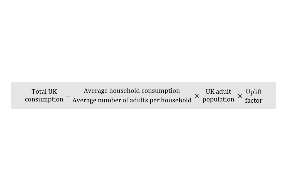
E9. Average adult consumption is estimated by dividing average household consumption by the average number of adults in a household. This is then converted into total UK consumption by multiplying by the UK adult population and then applying an uplift factor.
Living Costs and Food Survey
E10. The average weekly expenditure on spirits and beer for UK households is estimated using the LCF. Households participating in the surveys are asked to record their expenditure on alcohol under the relevant specific category of drink (that is wine, spirits, beer, etc.). There is an additional category for recording drinks purchased as part of a ‘round’ of drinks, which will be referred to as ‘other drinks’.
E11. Some of the ‘other drinks’ purchased will be spirits or beer. The calculation for consumption therefore includes a proportion of ‘other drinks’ purchases.
E12. The average weekly expenditure per household is converted to the volume consumed by that household using the average price of spirits/beer. This is then scaled up to an annual figure.
E13. The average consumption of spirits/beer per household is then converted to the average per person, by dividing by the average number of adults in a household. This is scaled up to the UK adult population.
E14. Most under-age drinking is taken into account in the alcohol models. We assume that adults buy most of the alcohol consumed by minors. This under-age alcohol expenditure is therefore included in the adults’ alcohol consumption and is measured by the survey.
E15. Due to the relatively small sample size in the LCF, the average weekly expenditure for spirits or beer is heavily influenced by extreme expenditure values in the data. Outliers in the data have been capped at the 99th percentile.
Cross-border and duty-free shopping
E16. Duty-free is included in the cross-border shopping calculation. Estimates of consumption of goods purchased as cross-border shopping are based on figures produced from the International Passenger Survey (IPS). This provides estimates of the volume of spirits and beer an average adult traveller brings into the country, separately for air and sea passengers. The IPS figures are weighted by the ONS, scaling up the survey data to represent the total cross-border shopping entering the UK.
E17. An estimate of the volume of duty-free spirits/beer brought into the country is calculated in the same way, using passengers coming from outside the European Union (EU).
E18. This estimate, however, does not cover sales made on-board ferries, so commercially provided data about deliveries of spirits/beer to ferries are used to supplement the cross-border shopping estimate, and provide a complete figure.
E19. Cross-border shopping is estimated as goods bought overseas, plus goods bought on-board ferries, plus duty-free.

E20. For tax year 2020 to 21, estimates of cross-border shopping and duty-free sales have been partially projected due to the IPS being suspended from March 2020 until December 2020 as a result of COVID-19 restrictions. The projection methodology calculates a 3-year average of cross-border and duty-free alcohol expenditure (based on latest available IPS data from 2017, 2018 and 2019). This 3-year average is applied to ONS published statistics on visitor numbers to and from the UK and their subsequent total expenditure where IPS data is not available in quarters 2, 3 and 4 of tax year 2020 to 2021.
Estimating legitimate consumption
E21. Legitimate consumption is calculated as UK duty paid consumption plus cross-border shopping.

E22. Estimates of UK duty paid consumption are taken directly from returns to HMRC of the volumes of spirits/beer on which duty has been paid. Duty is payable once alcoholic goods are released onto the UK market for consumption. Amounts released are referred to as ‘clearances’. For spirits the volumes of ready-to-drink products have been removed from spirits clearances in order to obtain figures for spirits only.
E23. Cross-border shopping is calculated in the same way as for total consumption: goods bought overseas, plus goods bought on-board ferries, plus duty-free.

Estimating the illicit market
E24. Total consumption is the sum of cross-border shopping (as defined in E19) and total consumption of UK purchases (as defined in E9). The illicit market volume is calculated by subtracting legitimate consumption (as defined in E21) from total consumption.

Conversion to monetary losses
E25. Revenue losses associated with the illicit market are then estimated by combining the illicit market share information with price data and duty and VAT rate information. The duty portion is calculated as illicit market volume, multiplied by spirits/beer duty rates. This is summed with the VAT portion, which is calculated as illicit volume, multiplied by average price, multiplied by the VAT fraction.
E26. Data on average spirits/beer prices is derived from data provided by the ONS. The prices used in the model are weighted across on-licence and off-licence and for different types of spirits/beer.
E27. The VAT fraction is the portion of the retail price that is VAT – for example, a 20% VAT rate is equivalent to a one-sixth VAT fraction. VAT fractions are calculated annually to capture changes in the VAT rate. This method assumes that VAT is also lost on all purchases. As, in some cases, the final illicit product is sold in legitimate outlets this may not always be the case, and this will be an overestimate of revenue losses.
E28. For the spirits calculation, spirits duty is converted into bulk duty liabilities based on the assumption that spirit’s strength is constant at 38%.
Spirits uplift factor
E29. The LCF Survey data for alcohol are subject to under-reporting, they may under-represent certain sub-populations with a high average alcohol consumption, and do not cover the full extent of the alcohol market so an uplift factor is necessary to correct for these biases. This uplift factor is calculated by taking estimates of consumption from the LCF Survey in the base year and comparing these with independent estimates of total consumption.
E30. To do this we take a year in which there is believed to be little or no illicit market and use HMRC clearance data as a true indication of total consumption. In order to reduce sampling error, the uplift factor is derived by taking the average of 3 years of data from the base years: 1990 to 1991, 1991 to 1992 and 1992 to 1993.
E31. Separate uplift factors are calculated for on-licence and off-licence markets, and the formula is defined as legitimate consumption in the base years, divided by estimated total consumption in the base years.

E32. The uplift factors for on-licence and off-licence are 3.5 and 2.0 respectively.
Beer Uplift factor
E33. The basis for this uplift factor is the same as for spirits, an average of the 3 base years is used where there is assumed to be no illicit market. However due to the variation in price between draught and packaged beer, a different uplift factor to spirits is required.
E34. To calculate uplift factors for draught and packaged beer, LCF Survey data is split between on-licence and off-licence markets and then into draught and packaged beer. This uses market shares estimated from ONS and British Beer and Pub Association (BBPA) data.
E35. The base year uplift factors are defined as legitimate consumption in the base years, divided by estimated total consumption in the base years.

E36. An additional uplift for packaged beer is calculated, which varies year-on-year. This assumes that there is no or a negligible illicit market in draught beer, whereby consumption is equal to clearances in every year. The draught beer uplift and base year uplifts are combined to compute the packaged beer uplift. This is achieved by multiplying the draught uplift in the year of estimation by the ratio of packaged to draught uplifts in the base years.

E37. For tax year 2020 to 2021, the packaged beer uplift factor has been projected based on an average of the previous 3 years, resulting in a 2.8 uplift. This is due to model sensitivities around COVID-19 impacts on the LCF and BBPA data.
Removing spirit-based ready-to-drinks
E38. Spirit-based ready-to-drinks (RTDs) are packaged beverages that are sold in a prepared form, ready for consumption, such as alcopops.
E39. The LCF survey expenditure data for spirits includes expenditure on RTDs.
E40. RTDs are currently included in the ‘other excise duties’ estimates, so are removed from the spirits tax gap to avoid double counting. To remove RTDs, we estimate the proportion of total expenditure attributable to ready-to-drinks using data on expenditure from the ONS, and total pure alcohol clearances on spirits and RTDs from HMRC clearances.
Upper and lower confidence intervals in the spirits estimate
E41. The variation in the LCF is used to construct 95% confidence intervals around the central estimate. They indicate the potential size of chance fluctuations in the estimate due to sampling error. They do not take into account systematic error from the model assumptions in the central estimate.
Smoothing spirits total consumption
E42. The number of LCF responses reporting spirits expenditure is small relative to the survey’s sample size and so estimated average household expenditure can vary substantially between years. A 3-year rolling average is applied to the final total consumption estimate for spirits to reduce this volatility and make clearer the tax gap trend.
E43. The spirits tax gap estimate for the tax year 2020 to 2021 however has been projected based on the illicit market share for 2019 to 2020, as we do not have enough data to produce a 3-year rolling average. This estimate will be revised in the next edition and will be based on a rolling average of 3 years when 2021 to 2022 data is made available.
Beer lower estimate
Overview
E44. The beer tax gap lower estimate is produced using a bottom-up methodology. This means estimates of the illicit market are made directly, by estimating the fraud components that make up the illicit market. The following types of illicit beer are included in the lower estimate:
-
diversion of UK-produced beer
-
drawback fraud
E45. Some of this illicit beer is recovered through HMRC compliance activity, so this is subtracted to give the net tax gap. The tax gap estimate is defined as diversion of UK produced beer, plus drawback fraud, minus seizures of illicit beer.

E46. A number of beer fraud channels are not included in this methodology as we are currently unable to estimate them. This is one of the reasons it is a lower bounding estimate. These include:
-
smuggled beer
-
diversion of foreign produced beer
-
counterfeit beer
-
any other fraud we do not know about
Diversion of UK-produced beer
E47. Diversion fraud occurs when beer is moved in duty suspense to the EU and is subsequently diverted back into the UK under the cover of false documentation. The taxes are not declared on the beer and the illicit product enters the UK market.
E48. We estimate that diversion fraud is equal to the amount of beer moved in duty suspense from the UK to certain EU member states, minus legitimate demand for UK branded beer in those countries. That is, we assume that any UK beer which is not feeding demand abroad will be diverted back to the UK illicit market.

E49. The total amount of beer moved in duty suspense from the UK to the EU includes dispatches from both excise warehouses and brewers. Dispatches from excise warehouses are taken directly from Excise Warehouse Returns (W1 form). Dispatches from brewers are estimated using data from Beer Duty Returns (EX46 form). Total beer dispatches are calculated by summing warehouse and brewer dispatches.

E50. Brewers return data is used for dispatches (movements to EU countries) and exports (movements to non-EU countries) and it cannot be disaggregated. So, to estimate dispatches from brewers, we subtract an estimate of exports from brewers.

E51. Exports from brewers are estimated as total exports, from Customs Handling of Import and Export Freight (CHIEF), minus exports from Excise Warehouse Returns (W1 form).

E52. To preserve the lower bounding nature of this estimate, we only include dispatches to certain EU countries. These countries have been selected based on a number of factors, including: proximity to the UK; the differential in price; operational indications of risk and patterns of supply.
E53. The estimate of beer dispatches, described in paragraph E48 and E50, cannot be broken down to the recipient country. Therefore, we use an alternative data source, UK trade data, which does include a breakdown by country. The proportion of beer dispatched to the selected EU countries is taken from UK trade data and applied to the estimated total dispatches to produce an estimate for dispatches to these selected EU countries.
E54. UK trade data is not used to directly estimate dispatches to these countries as it does not include certain types of movements. More detail is provided on this in paragraph E68.
E55. To summarise, total duty suspended beer moved to selected EU countries is calculated as the product of the percentage of dispatches going to selected EU countries (as defined in E53) and total dispatches to EU countries. Total dispatches to EU countries is defined as the sum of dispatches from warehouses and brewers. Dispatches from brewers must be calculated by subtracting the difference between total exports and warehouse exports from total dispatches and exports from brewers.

Drawback fraud
E56. Drawback fraud occurs when goods are moved to the EU and the duty is reclaimed via drawback. Duty is then paid at the lower rate in the destination country and the goods are illicitly returned to the UK.
E57. To estimate drawback fraud, we estimate the volume of beer corresponding to certain drawback claims, then subtract the legitimate demand for beer in the selected destination countries.

E58. To preserve the lower bounding nature of this estimate, we only include drawback if it is claimed for dispatch by a business not part of HMRC Large Business. The value of these drawback claims is converted to volume of beer by dividing by the average duty rate for beer.
E59. The volume is then adjusted using the proportion of dispatches going to the selected EU countries. This gives an estimate of the amount of beer going to the selected countries with drawback claimed by small and medium sized enterprises.

Legitimate demand in selected EU countries
E60. Some of the beer moved to the selected EU countries will be supplying legitimate demand within those countries, rather than being diverted to the UK illicit market. We make one overall estimate of legitimate demand in the selected EU countries and subtract it from the sum of selected beer dispatches and selected beer for drawback.
E61. We have purposely overestimated legitimate demand by only accounting for the riskiest countries, which produces an underestimate of the illicit market, in order to maintain the lower bounding nature of the tax gap estimate.
E62. The estimate of legitimate demand in other countries sums cross-border shopping bought by UK residents and legitimate consumption abroad. The latter may include:
-
consumption by UK expatriates
-
consumption by UK residents while abroad
-
consumption by foreign nationals
-
beer in transit to other countries

E63. Cross-border shopping is estimated using data from the IPS. More detail is provided in paragraph E16. Only passengers from the selected EU countries are included.
Legitimate consumption of UK produced beer abroad
E64. We could not find reliable data on legitimate consumption of UK produced beer abroad. So, we estimate it based on the assumption that in a certain year, when the illicit market upper estimate was low, there was negligible illicit activity meaning all dispatches to the selected EU countries were consumed legitimately. This is likely to provide an overestimate of legitimate consumption abroad, as there would likely be some level of fraud in these years. This supports the methodology being a lower estimate of the tax gap.
E65. For stability, an average of 2 years is used: 2000 to 2001 and 2001 to 2002. We refer to these 2 years as the ‘base year’.
E66. Brewers return data is not available for years prior to 2007. Consequently, we use an alternative data source, UK trade data, to estimate dispatches in the base year.
E67. In the base year we assume that all dispatches supply either cross-border shopping by UK residents or legitimate consumption abroad. We subtract an estimate of cross-border shopping in the base year from dispatches in the base year; the remainder is assumed to be legitimate consumption abroad.

E68. We believe that UK trade data may underestimate beer dispatches in the base year as it does not record certain types of beer movement. These include:
-
goods in transit
-
deliveries to embassies
-
deliveries to Navy, Army and Air Force Institutes (NAAFI)
E69. Additionally, as the threshold for recording goods on UK trade data is relatively high, beer may have a higher proportion of small traders than other commodities. This may mean the standard adjustment applied to UK trade data to account for small traders may be too low for beer.
E70. To account for these concerns, we uplift the UK trade data. There is very little evidence to indicate the actual scale of uplift required. Comparison with our calculated dispatches in later years led us to apply a factor of 2. Again, the high level of this adjustment may result in this being an overestimate of legitimate demand. This is in keeping with the lower bounding methodology for the tax gap, as higher legitimate demand would see a lower estimate for the illicit market.
Illicit market lower estimate
E71. To summarise, the beer illicit market lower estimate is calculated by summing selected dispatches (as defined in E55) and selected drawback (as defined in E58 and E59), before subtracting seizures of illicit beer and legitimate demand in selected countries. Legitimate demand in selected countries is defined as cross-border shopping (CBS) of UK residents plus legitimate consumption abroad (as defined in E67).

E72. Since the tax year 2016 to 2017, the beer illicit market lower estimate has been projected to better reflect changes in fraud. This is calculated by keeping the gross tax gap constant, whilst using operational intelligence as a proxy to capture the impact of changes in the illicit market.
Implied mid-point estimate
E73. The implied mid-point estimate is calculated as the average of the upper and lower estimates. It is only intended as an indicator of long-term trend – the true tax gap could lie anywhere within the bounds.
E74. The bounds do not take account of any systematic tendency to over- or under-estimate the size of the tax gap that might arise from the modelling assumptions.
Wine central estimate
E75. We have not estimated the illicit market share for wine due to the unavailability of a key commercial data source previously used to estimate the wine tax gap. We therefore include wine within our tax gap estimate for ‘Other taxes, levies and duties’, which is based on an experimental method. See ‘Chapter J: Other taxes’.
Chapter F: Tobacco
Overview
F1. The estimate of the illicit market for tobacco is produced using a top-down methodology. That is, first we estimate total consumption, and then we subtract legitimate consumption. The residual is estimated to be the volume of goods supplied through the illicit market.

F2. This residual is then turned into an estimate of the proportion of the total market that is supplied through the illicit market by dividing illicit market volume by total consumption volume and then multiplying by 100 to convert it into a percentage. This is termed the illicit market share.

F3. Revenue losses associated with the illicit market are then estimated by combining the illicit market share information with price data, excise duty, and VAT rate information.
Methodology
F4. The estimates of the illicit market for cigarettes and hand-rolling tobacco are produced using a top-down methodology as described in paragraphs F1 to F3. These estimates combined provide the tobacco tax gap.
F5. Details of the estimation of total consumption and of legitimate consumption are provided in the subsequent sections.
F6. Due to changes to the Office for National Statistics’ Opinions and Lifestyle Survey (OPN), which is used to estimate total consumption, the cigarette and hand-rolling tobacco tax gaps from quarter 4 of the 2017 to 2018 tax year have been projected.
F7. For quarter 4 of 2017 to 2018, we have assumed the average daily consumption to be consistent with quarter 4 of 2016 to 2017. This method is different to that set out in F8 as we only needed to project one quarter.
F8. For 2018 to 2019 onwards, we have assumed the percentage tax gaps for cigarettes and hand-rolling tobacco to be the same as 2017 to 2018. Whilst the tax gap percentages have been kept static since 2017 to 2018, we have still used actual clearances in the tax gap calculations, which means that total consumption will be scaled accordingly. Amounts released are referred to as ‘clearances’, which is when duty is payable once alcoholic goods are released onto the UK market for consumption.
F9. The methodology used for tax years up to and including 2016 to 2017 are based on the descriptions set out from F10. The calculations on legitimate consumption apply to all years.
Total consumption
F10. The total consumption in any given year is calculated using the following:
-
estimates of prevalence (proportion of the population that smoke cigarettes) from the General Lifestyle Survey (GLF), the Opinions and Lifestyle Survey (OPN) and Health Survey for England (HSE)
-
estimates of cigarette consumption per smoker from GLF, OPN and HSE
-
estimates of the adult population (ages 16 or over) from the Office for National Statistics (ONS)
-
an uplift factor covering under-reporting
F11. The estimate of total UK cigarettes and hand-rolling tobacco consumption for each year is a product of the estimates of cigarette and hand-rolling tobacco smoking prevalence and consumption per smoker for declared and undeclared smokers.
F12. In general, most smokers admit that they smoke and so we can obtain the prevalence and consumption per smoker of these declared smokers from the OPN since 2012. There are some smokers who, for whatever reason, do not admit that they smoke. We therefore obtain the undeclared smokers in the non-smoking population from the HSE.
Uplift factor
F13. We expect that tobacco consumption is under-reported in social surveys such as the OPN, which may be due to reasons such as social desirability that can influence participants’ responses. We apply an uplift factor to correct for this bias. This uplift factor is calculated by taking estimates of total consumption from the GLF in a base year. In cigarettes the base year is 1996 to 1997, and in hand-rolling tobacco it is an average of 3 years, 1983 to 1986. Estimates of total consumption in base years are compared with consumption of actual clearances to HMRC and an estimate of legitimately purchased cigarettes from abroad.

F14. The uplift factors for the 2020 to 2021 cigarettes and hand-rolling tobacco estimates are 1.5 and 1.1 respectively. These were calculated from the base year by taking legitimate consumption (from HMRC clearances and an estimate of duty-free/cross-border shopping) divided by total consumption (based on self-reported consumption from the GLF survey).
Upper and lower bounds for total consumption
F15. The uncertainties in the survey data used to create these estimates mean that it is not possible, with sufficient accuracy, to produce a single point estimate of total consumption. However, due to the methodology we use, it is difficult to produce confidence intervals. Instead, we use the survey data to produce an upper bound and lower bound for total consumption. This allows us to produce a range for total consumption that takes account of the uncertainty in the underlying data.
F16. The one difference between the upper and lower bound calculations is the treatment of dual smokers. Dual smokers are individuals who consume both cigarettes and hand-rolling tobacco. In the upper bound calculation, the majority of the dual smokers are considered to be cigarette smokers. In the lower bound estimate, we assume that the majority smoke hand-rolling tobacco. This is explained further in the following tables and sections.
Table F.1 Cigarettes upper and hand-rolling tobacco lower bound assumptions
| Allocation of total tobacco consumption for estimates | Allocation of total tobacco consumption for estimates | |
|---|---|---|
| OPN Survey Options | Cigarette upper bound assumption | Hand-rolling tobacco lower bound assumption |
| Cigarettes only | 100% | 0% |
| Dual smokers: cigarettes and hand-rolling tobacco, but mainly cigarettes | 99% | 1% |
| Dual smokers: cigarettes and hand-rolling tobacco, but mainly hand-rolling tobacco | 49% | 51% |
| Hand-rolling tobacco only | 0% | 100% |
Table F.2 Cigarettes lower and hand-rolling tobacco upper bound assumptions
| Allocation of total tobacco consumption for estimates | Allocation of total tobacco consumption for estimates | |
|---|---|---|
| OPN Survey Options | Cigarette lower bound assumption | hand-rolling tobacco upper bound assumption |
| Cigarettes only | 100% | 0% |
| Dual smokers: cigarettes and hand-rolling tobacco, but mainly cigarettes | 51% | 49% |
| Dual smokers: cigarettes and hand-rolling tobacco, but mainly hand-rolling tobacco | 1% | 99% |
| Hand-rolling tobacco only | 0% | 100% |
F17. The upper bound of total cigarette or hand-rolling tobacco consumption is calculated firstly by estimating consumption levels from smokers who only smoked cigarettes or hand-rolling tobacco . This is added together with a maximum consumption of cigarettes or hand-rolling tobacco that could be smoked by dual smokers.
F18. The lower bound of total cigarette or hand-rolling tobacco consumption is calculated firstly by estimating consumption levels from smokers who only smoked cigarettes or hand-rolling tobacco. This is added together with a minimum consumption of cigarettes or hand-rolling tobacco that could be smoked by dual smokers.
F19. Tobacco tax gap estimates up to and including quarter 3 of 2011 to 2012 use the GLF as the base estimate for tobacco consumption. These estimates are supplemented with OPN data on dual smokers where this is added/subtracted to obtain the upper and lower bounds. All years from quarter 4 of 2011 to 2012 are based on OPN data only.
Legitimate consumption
F20. Estimates of legitimate consumption include:
-
UK duty paid consumption
-
cross-border and duty-free shopping
UK duty paid consumption
F21. Estimates of UK duty paid consumption are taken directly from tax returns to HMRC (clearance data) on the volumes of cigarettes and hand-rolling tobacco on which duty has been paid, along with the actual amounts of money.
Cross-border and duty-free shopping
F22. Estimates of consumption of goods purchased as cross-border shopping are based on data from the International Passenger Survey (IPS). This provides estimates of the number of cigarettes and/or hand-rolling tobacco that an average adult traveller brings into the country, separately for air and sea passengers. The IPS figures are weighted by the ONS, scaling up the survey data to represent the total cross-border shopping entering the UK.
F23. This estimate, however, does not cover sales made on-board ferries. Commercially provided data about deliveries of cigarettes to ferries is used to supplement the cross-border shopping estimate.
F24. Duty-free cigarettes/hand-rolling tobacco brought into the UK are also estimated from the IPS, using passengers coming back from outside the EU.
F25. Legitimate consumption is estimated as UK duty paid consumption, plus cross-border shopping, plus duty-free.

F26. For tax year 2020 to 21, estimates of cross-border shopping and duty-free sales have been partially projected due to the IPS being suspended from March 2020 until December 2020 as a result of COVID-19 restrictions. The projection methodology calculates a 3-year average of cross-border and duty-free tobacco expenditure (based on latest available IPS data from 2017, 2018 and 2019). This 3-year average is applied to ONS published statistics on visitor numbers to and from the UK and their subsequent total expenditure where IPS data is not available in quarters 2, 3 and 4 of tax year 2020 to 2021.
Conversion to monetary losses
F27. All calculations to this point have been made on volumes of cigarettes or hand-rolling tobacco. Revenue losses associated with the illicit market are then estimated by combining the illicit market share information with price data, duty, and VAT rate information. Volumes are converted to estimates of revenue losses by multiplying by the sum of specific duty and ad valorem liabilities. Ad valorem liabilities are calculated as average price multiplied by the sum of ad valorem duty and the VAT fraction. Ad valorem taxes and duties are applied to transactions and are levied in relation to the assessed value of the good.

F28. The average price is taken as the weighted average price (WAP) of all cigarettes or hand-rolling tobacco that were UK duty paid. The WAP is calculated by weighting the retail price of each product by the share of clearances in the cigarette or hand-rolling tobacco market.
F29. The VAT fraction is the proportion of the retail price that is VAT – for example, a 20% VAT rate is equivalent to one-sixth VAT fraction. VAT fractions are calculated annually to capture changes in the VAT rate. This method assumes that VAT is also lost on all purchases. In some cases, the final illicit product is sold in legitimate outlets where VAT is paid, so this method results in an overestimate of revenue losses.
Summary of cigarette methodology
F30. In summary, the illicit market for cigarettes is calculated as the sum of declared and undeclared consumption, minus legitimate consumption.
F31. Declared consumption is defined as the total adult population, multiplied by the uplift factor, multiplied by the sum of declared consumption by cigarettes and dual smokers. The upper bound assumes most dual smokers smoke cigarettes, whilst the lower bound assumes most smoke hand-rolling tobacco. Undeclared consumption is defined as the product of the non-smoker population, the uplift factor, the under-declared smokers prevalence and the consumption per under-declared smoker.
F32. Legitimate consumption is defined as UK duty paid consumption (from HMRC clearance data), plus cross-border shopping (the sum of on-board ferry sales and the average amount per traveller, multiplied by the number of travellers), plus duty-free (from the IPS).

Summary of hand-rolling tobacco methodology
F33. In summary, the illicit market for hand-rolling tobacco is calculated as the sum of declared and undeclared consumption, minus legitimate consumption.
F34. Declared consumption is defined as the total adult population, multiplied by the uplift factor, multiplied by the sum of declared consumption by hand-rolling tobacco and dual smokers. The upper bound assumes most dual smokers smoke hand-rolling tobacco, whilst the lower bound assumes most smoke cigarettes. Undeclared consumption is defined as the product of the non-smoker population, the uplift factor, the under-declared smokers prevalence and the consumption per under-declared smoker.
F35. Legitimate consumption is defined as UK duty paid consumption (from HMRC clearance data), plus cross-border shopping (the sum of on-board ferry sales and the average amount per traveller, multiplied by the number of travellers), plus duty-free (from the IPS).

Chapter G: Diesel
Methodology
G1. A bottom-up methodology is used to estimate the diesel tax gap from the tax year 2016 to 2017 onwards based on a random enquiry programme. The Great Britain (GB) and Northern Ireland (NI) diesel tax gaps are calculated separately but the methodologies are identical.
G2. Figures prior to 2016 to 2017 are calculated using a top-down methodology based on road statistics. This methodology was no longer fit for purpose from the tax year 2013 to 2014 as it was not sensitive enough to accurately measure the low tax gap. This meant the estimates for 2013 to 2014 were rolled forward for 2014 to 2015 and 2015 to 2016 before a bottom-up approach was introduced in 2016 to 2017.
G3. Since previous years are based on a top-down methodology, figures from 2016 to 2017 onwards are not directly comparable to these.
G4. The methodology below describes the bottom-up approach used from 2016 to 2017.
G5. Summary of methodology:
-
legitimate consumption is based on the returns that HMRC receives from the volumes of diesel on which duties have been paid (HMRC clearances)
-
illicit consumption is estimated using the proportion of vehicles found to be misusing rebated fuel in random sample surveys conducted by HMRC in 2017 and 2020
-
revenue losses (gross tax gap) associated with illicit consumption are estimated using average retail prices, duty rates and VAT rates
-
the net tax gap is then calculated as the gross tax gap minus compliance yield
Estimating total consumption
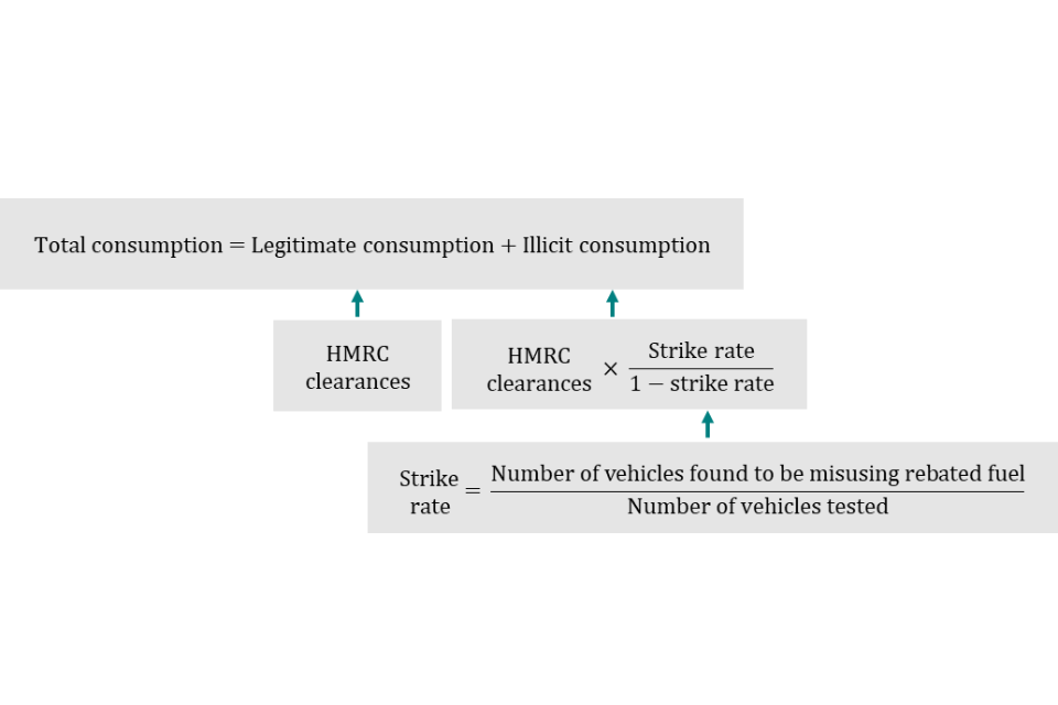
G6. Total consumption is calculated as legitimate consumption plus illicit consumption.

G7. HMRC conducted random surveys in April to June 2017 and January to March 2020 where vehicles were stopped at the roadside and tested for illicit diesel. In both surveys, a stratified sample of 1,900 vehicles across the UK (1,500 in GB and 400 in NI) was used. The sample was stratified by vehicle type and region to ensure the results were representative of all vehicles across the UK.
G8. The proportion of vehicles found to be misusing rebated fuel in each survey is referred to as the strike rate, which is calculated by taking the number of vehicles found to be misusing rebated fuel divided by the number of vehicles tested. The strike rate is used as an estimate of the proportion of vehicles misusing rebated fuel in the UK.

G9. The strike rate is then used alongside legitimate consumption to give estimates for total and illicit consumption. A separate strike rate is calculated in each survey for GB and NI. The strike rate created using 2017 survey data is used for tax years 2016 to 2017, 2017 to 2018 and 2018 to 2019, with the 2020 survey strike rate used for tax years 2019 to 2020 and 2020 to 2021.
G10. To calculate total diesel consumption, we add legitimate consumption and illicit consumption. Legitimate consumption is made up of HMRC clearances. Illicit consumption is defined as the product of HMRC clearances, and the strike rate (defined in G8) divided by one minus the strike rate.
Conversion to monetary losses
G11. The diesel tax gap is driven by the misuse of rebated fuel. Rebated fuel is subject to a lower duty rate and has a lower retail price including VAT. Revenue loss occurs where this fuel is misused, and so should have been subject to a higher rate of fuel duty and additional VAT.
G12. In order to estimate the revenue losses associated with the misuse of rebated fuel, the duty and VAT paid needs to be taken into account. Therefore, the difference between rebated and un-rebated duty rates has been used to estimate the duty loss associated with the illicit market.
G13. Similarly, the difference in average retail prices for rebated fuel and un-rebated diesel has been used to estimate the VAT loss associated with the illicit market. Published data from the Department for Business, Energy and Industrial Strategy (BEIS) has been used to calculate average retail prices.
G14. These calculations provide the revenue losses associated with illicit consumption, which we describe as the gross tax gap.
G15. The net tax gap is then calculated as the gross tax gap minus compliance yield.
Confidence intervals
G16. The upper and lower estimates correspond to confidence intervals that indicate the range where the true value of the illicit market may lie and arises due to random sampling error in calculating the strike rate.
Exclusions
G17. Smuggling and laundering of diesel is excluded on the basis that it is believed to be a smaller issue compared to the misuse of rebated fuel, the scale of which isn’t currently quantifiable. Cross-border shopping is excluded due to a reduced-price difference between the Republic of Ireland and NI, meaning there is limited motivation for cross-border shopping activities. Revenue losses are assumed to be related to the misuse of gas oil (red diesel) only. The misuse of other fuels (for example, kerosene) has been excluded on the basis that this is believed to be a minor issue, the scale of which isn’t currently quantifiable.
Chapter H: Estimates using random enquiry programmes (REP)
H1. This chapter covers all the approaches taken to produce Income Tax, National Insurance contributions (NICs) and Capital Gains Tax (CGT) gaps as well as the small business Corporation Tax and small business Employer Compliance (EC) gaps. The EC gap for large business employers is based on historical trends in the small business gap, the details of this are described in paragraph H61.
Random enquiry programme estimates
H2. There are 3 direct tax random enquiry programmes (REP) which are used to produce tax gap estimates. They cover:
-
Self Assessment individuals and small partnerships
-
small business employers
-
Corporation Tax for small businesses
H3. Random enquiry programmes allow HMRC to estimate the extent of under-declaration of liabilities arising from the submission of incorrect returns. Each return selected is subject to a full enquiry involving a complete examination of records. Under certain circumstances, a full enquiry may not take place if the return can be verified through third party information.
Populations and sampling
H4. The sizes of the samples for the 3 programmes are shown in Tables H.1, H.2 and H.3 below.
Table H.1: Sample sizes for the Self Assessment random enquiry programme
| Self Assessment - Tax return year | Self Assessment - Sample size |
|---|---|
| 2005 to 2006 | 5,234 |
| 2006 to 2007 | 2,925 |
| 2007 to 2008 | 2,864 |
| 2008 to 2009 | 2,708 |
| 2009 to 2010 | 2,116 |
| 2010 to 2011 | 2,033 |
| 2011 to 2012 | 2,251 |
| 2012 to 2013 | 2,193 |
| 2013 to 2014 | 2,042 |
| 2014 to 2015 | 1,771 |
| 2015 to 2016 | 2,091 |
| 2016 to 2017 | 2,255 |
| 2017 to 2018 | 1,804 |
| 2018 to 2019 | — |
| 2019 to 2020 | — |
| 2020 to 2021 | — |
Note for Table H.1
- Sample size figures from 2010 to 2011 onwards have been adjusted due to reclassifying some cases as being within the population of interest.
Table H.2: Sample sizes for employer compliance random enquiry programme
| Employer Compliance - Tax return year | Employer Compliance - Sample size |
|---|---|
| 2005 to 2006 | 1,285 |
| 2006 to 2007 | 1,184 |
| 2007 to 2008 | 1,077 |
| 2008 to 2009 | 1,174 |
| 2009 to 2010 | 1,180 |
| 2010 to 2011 | 496 |
| 2011 to 2012 | 653 |
| 2012 to 2013 | 665 |
| 2013 to 2014 | 751 |
| 2014 to 2015 | 766 |
| 2015 to 2016 | 714 |
| 2016 to 2017 | 619 |
| 2017 to 2018 | 670 |
| 2018 to 2019 | 667 |
| 2019 to 2020 | 622 |
| 2020 to 2021 | 663 |
Note for Table H.2
- Since the tax year 2015 to 2016 the Employer Compliance sample size given is for small business only. Before 2015 to 2016 HMRC’s former small and medium-sized enterprises (SME) customer group classification was used.
Table H.3: Sample sizes for Corporation Tax random enquiry programme
| Corporation Tax - Accounting period ending in year | Corporation Tax - Sample size |
|---|---|
| 2005 to 2006 | 419 |
| 2006 to 2007 | 460 |
| 2007 to 2008 | 492 |
| 2008 to 2009 | 491 |
| 2009 to 2010 | 480 |
| 2010 to 2011 | 490 |
| 2011 to 2012 | 567 |
| 2012 to 2013 | 671 |
| 2013 to 2014 | 540 |
| 2014 to 2015 | 583 |
| 2015 to 2016 | 362 |
| 2016 to 2017 | 364 |
| 2017 to 2018 | 342 |
| 2018 to 2019 | — |
| 2019 to 2020 | — |
| 2020 to 2021 | — |
Note for Table H.3
- Since the tax year 2016 to 2017 the Corporation Tax sample size given is for small business only. Before 2016 to 2017 HMRC’s former small and medium-sized enterprises (SME) customer group classification was used.
H5. To produce population estimates for total tax gaps from the samples in Tables H.1, H.2 and H.3, the average tax gap estimates from random enquiries are multiplied by the number of taxpayers in the population.
H6. Adjustments are made to the population for cases deselected because they are outside of the population of interest, for example, the business is no longer operating or is part of the large business customer group.
Self Assessment
H7. The Self Assessment random enquiry programme allows us to estimate the tax gap arising from under-declaration of tax liabilities of individuals in Self Assessment and is used in conjunction with operational enquiry data. Results from enquiries are scaled up to the total number of individuals who are sent a Self Assessment notice to file and who are in the population of interest. For individuals not covered by the random enquiry programme, operational enquiry data is used. Further details regarding this data are given in the ‘Enquiry data’ section of this chapter.
H8. In this context, ‘individuals’ means individuals who are self-employed, pensioners, and partnerships (with up to 4 partners), as well as those who are employees or may only have investment income. The taxes directly included are:
-
Income Tax
-
National Insurance contributions
-
Capital Gains Tax
H9. The random sample used for the programme is selected from Self Assessment taxpayers issued with a notice to file a return. The sample is drawn by a systematic process that selects every “nth” notice. The sampling interval, n, is determined by dividing the total number of returns issued by the required sample size (rounded down to the nearest whole number). When a non-business taxpayer’s return includes a partnership income schedule, and no other income, reliefs or charges, we deselect that return. This is because the returns of individuals who are partners will automatically be included in any enquiry resulting from the selection of a partnership return.
H10. 2009 to 2010 is the last year which uses a simple random sample, as random samples for subsequent years have been stratified to improve the accuracy of the results. Samples drawn from Self Assessment business taxpayers are stratified by turnover from 2010 to 2011 onwards, with samples drawn from Self Assessment non-business taxpayers stratified by level of income from 2011 to 2012 onwards.
H11. From 2015 to 2016 we used an optimal allocation method in order to increase the accuracy of our estimates. When sampling, we take into account the variability of the tax at risk across the strata in the population. We select a greater proportion of cases in strata where the variance of tax at risk values is known to be high.
H12. Self Assessment business consists of the self-employed and partnerships. Self Assessment non-business consists of employees, pensioners, trusts and all other types of Self Assessment taxpayers. In order to improve how representative the sample is, weighting is applied based on how these customer groups are distributed across the population for the relevant tax year. We continue to review the customer group population assumptions.
H13. Due to a relatively small sample size and large natural variance in the levels of under-declared liabilities from year to year, a smoothing approach has been used for small partnerships from 2010 to 2011 (when the stratification of business taxpayers was introduced). A 3-year moving average with a double weighting given to the current year is used to smooth the data. This ensures that the resulting estimates are less susceptible to sampling variability and more indicative of longer-term trends.
H14. When using random enquiry programme data, we forecast the results of incomplete cases. The forecasts for open cases will be replaced with settlement data once available, which may lead to revisions to the estimate in future editions of ‘Measuring tax gaps’.
Employer compliance
H15. The employer compliance (EC) random enquiry programme allows us to estimate the tax gap arising from Pay As You Earn (PAYE) failures and other irregularities. Results from the EC random enquiry programme are scaled up to the total number of PAYE schemes.
H16. The employer may be an individual, partnership, public body, charity, or a company and will be required to make returns under the PAYE regulations to account for Income Tax and NICs.
H17. The figures relate to Income Tax, NICs, and Student Loan Repayments collected through PAYE due on earnings and other income from employment. The scope of these figures also includes tax due on occupational pensions taxed through PAYE.
H18. The random sample is selected using the former small and medium-sized enterprises (SME) customer classification and stratified on the basis of employer characteristics (defined in terms of the number of employees and whether the employer’s business is incorporated). Prior to ‘Measuring tax gaps 2020’ edition we calculated the small business tax gap by first calculating the EC tax gap for SME employers. This SME estimate was then converted to a small business estimate using historical data on tax receipts that was available under both groupings.
H19. From ‘Measuring tax gaps 2020 edition’ the EC small business tax gap is calculated directly using small business only data for the tax year 2015 to 2016 and onwards. This is done by flagging and removing mid-sized businesses from the random sample to create a small business only sample. However, for historical years the conversion factor is still applied as the source data does not contain the information required for the identification of mid-sized businesses, therefore they cannot be removed.
Corporation Tax
H20. The Corporation Tax random enquiry programme allows us to estimate the tax gap arising from incorrect Corporation Tax returns of small businesses. Results from the Corporation Tax random enquiry programme are scaled up to the total number of live small business trader cases. In this context, ‘live’ excludes cases which are, for instance, dormant or dissolved. In addition to this, sample cases are excluded if the company has not submitted a return for the year of interest.
H21. For Corporation Tax, up to the tax year 2015 to 2016, the random sample was selected using the former SME customer classification. From 2016 to 2017 the random sample is selected from the small business customer group from businesses which have been issued a notice to file a return.
H22. The random enquiry programme data is used to directly calculate the Corporation Tax small business tax gap from the tax year 2016 to 2017 and onwards. For earlier years the random enquiry data was collected under the former SME population definition and the estimate of the small business tax gap was estimated by applying a conversion factor which was derived using historical data on tax receipts that was available under both groupings.
H23. From April 2013, we changed the sampling process to a stratified random sample, based on the size of annual trading turnover. This change allowed the Corporation Tax random enquiry results to be weighted by the actual population of each stratum resulting in improved accuracy of the tax gap results.
H24. Due to a relatively small sample size and large natural variance in the levels of under-declared liabilities from year to year, a smoothing approach is used. A 3-year moving average with a double weighting given to the current year is used to smooth the Corporation Tax small business data throughout the series. This ensures that the resulting estimates are less susceptible to sampling variability and more indicative of longer-term trends.
Data features
H25. The latest observed random sample for Self Assessment used in the ‘Measuring tax gaps 2022 edition’ estimates is for 2017 to 2018. More detail of the timing of random enquiries is given in the next section. From 2014 to 2015 approximately half of the sample was worked as a desk-based enquiry rather than the standard face to face approach before the move to a fully desk-based approach was implemented in the tax year 2016 to 2017. An evaluation of the effect of working random enquiry programme cases as a desk-based enquiry as opposed to face to face was carried out and found no statistically significant evidence that it affected the outcome of the enquiry.
H26. The latest observed EC random sample is for 2020 to 2021. From 2015 to 2016, approximately half of the sample was worked as a desk-based enquiry rather than a face to face approach before the move to a fully desk-based approach was implemented in the year 2018 to 2019. An evaluation of the effect of working cases as a desk-based enquiry as opposed to face to face was carried out and found no statistically significant evidence that it affected the outcome of the enquiry.
H27. The latest observed Corporation Tax random sample is for 2017 to 2018. This sample was originally split equally to evaluate the impact of working CT REP cases as desk-based enquiries as opposed to the standard face to face approach. However, all 2017 to 2018 CT REP cases were worked as a desk-based enquiry. This was due to the pandemic where all face to face enquiries were paused. The trial has resumed for Corporation Tax REP data relating to 2021 to 2022.
Timing
H28. There are 2 factors which influence the timing of the latest available tax gap estimate for a particular type of tax return:
-
delays inherent in the returns process; this varies according to the head of duty and is shown in Table H.4 below
-
delays due to the complexity of some random enquiries; it can take several years before sufficient random enquiries relating to a particular tax year are settled to robustly report the results
Table H.4: Comparison of delays due to returns process
| Random enquiry programme | Delays due to returns process |
|---|---|
| Self Assessment | Individuals generally have until 31 January following the year of assessment to which the return relates to submit their return. Once the return is submitted, HMRC then has a further year in which to open an enquiry. |
| Employer compliance | None. EC reviews initially look at the records of the previous 12 months. |
| Corporation Tax | Companies have until a year after the end of their accounting period to submit their return. HMRC then has a further year in which to open an enquiry. |
H29. There are consequences of the timing issues described above. Firstly, estimates of tax gaps for Corporation Tax and Self Assessment are not available for the latest years due to a lag in data available, so to present a more consistent picture of the scale of tax losses, projection factors have been applied to the estimates for Corporation Tax and Self Assessment. We use the latest available data to project future years as this allows us to most effectively reflect recent policy and other changes that have a long-term impact on taxpayer behaviour. These projection factors are shown below in Table H.5.
H30. Secondly, estimates for earlier years have been revised since previously published, as a result of the inclusion of additional data from enquiries that have since been completed. Finally, at the time of estimation, some enquiries across several years’ random enquiry programmes were not closed. In order to estimate tax gaps for each year, it is necessary to make assumptions about the cases that were yet to be settled at the date the enquiry results are analysed. Forecasts for such enquiries are made based on the results of recently settled enquiries with similar durations. Where possible, caseworker forecasts are also used.
H31. In ‘Measuring tax gaps 2022 edition’ there has been an adjustment to project the estimate of the Self Assessment tax gap over 3 years, an extra year compared to previous publications, due to increased REP uncertainties from different ways of working cases during the pandemic, to allow time for more 2018 to 2019 REP cases to close and to complete assurance/validation of the results.
H32. In ‘Measuring tax gaps 2022 edition’ there has been an adjustment to project the estimate of the Corporation Tax small business tax gap over 3 years, an extra year compared to previous publications, due to increased REP uncertainties from different ways of working cases during the pandemic, to allow time for more 2018 to 2019 REP cases to close and to complete assurance/validation of the results.
Table H.5: Comparison of projection factors
| Random enquiry programme | Projection factors |
|---|---|
| Self Assessment | For the years after 2017 to 2018 where we do not have random enquiry data, the latest available estimate is projected forward. The projections are made by keeping the percentage gross tax gap constant and using actual tax liabilities, non-payment and compliance yield for the relevant tax. |
| Corporation Tax | For the years after 2017 to 2018 where we do not have random enquiry data, the latest available estimate is projected forward. The projections are made by keeping the percentage gross tax gap constant and using actual tax liabilities, non-payment and compliance yield for the relevant tax. |
| Employer Compliance | No projection factor is used. |
Sources of error
H33. There are 2 main sources of error associated with the results of random enquiries which could result in the true values of the tax gaps differing from the estimates produced. These are:
-
sampling variation in the data: the whole population is not subject to enquiry, so even though the sample is designed to be representative, its characteristics may differ from the population purely by chance
-
systematic uncertainty where the sample results consistently tend to under-report the true values for the population, or where the sample does not include the full population, for example those participating in avoidance
H34. We make an adjustment for one source of systematic uncertainty, which is non-detection of non-compliance. The random enquiry programmes will not identify all incorrect returns or the full scale of under-declaration of liabilities, so estimates produced from the unadjusted results of the programmes would underestimate the full extent of the tax gap. The Internal Revenue Service (IRS) in the United States (US) has previously tackled this problem by using a range of ‘multipliers’ to adjust for non-detection. The principles behind the IRS methodology have been applied to HMRC’s data to produce approximate multipliers for the UK. The IRS report is available at IRS report - Tax Compliance.
H35. The IRS was able to undertake this analysis of non-detection because their random enquiry samples covered upward of 50,000 cases – much higher than is feasible in the UK. In the absence of much of this data for the UK, the US multipliers are mainly used to account for non-detection. The size of the multipliers varies by the type of non-compliance found and are consistent year-on-year; Table H.6 shows how these multipliers differ by each random enquiry programme.
H36. For Employer Compliance and Corporation Tax in Table H.6, specific non-detection multipliers have been derived using the ‘Delphi’ approach. More information about the Delphi approach and our plans to carry out a programme of development to introduce new non-detection multipliers in future editions of ‘Measuring tax gaps’ can be found in HMRC’s working paper ‘Non-detection multipliers for measuring tax gaps’. We use symmetrical upper and lower bounds for illustrative purposes, where they do not feed into the overall tax gap figure. Our lower bound is fixed at 1 for all regimes under an assumption that all non-compliance is detected by HMRC.
Table H.6: Comparison of adjustments for non-detection
| Random enquiry programme | Multiplier for central estimate | Multiplier for lower estimate | Multiplier for upper estimate |
|---|---|---|---|
| Self Assessment (business) | 1.908 | 1.000 | 3.075 |
| Self Assessment (non-business) | 1.260 | 1.000 | 1.928 |
| Employer compliance | 1.200 | 1.000 | 1.400 |
| Corporation Tax | 1.457 | 1.000 | 1.914 |
Validation
H37. As part of each year’s programme, HMRC conducts a validation exercise for a sample of cases. These cases are checked to confirm that the enquiry outcomes (for example, the amount of yield) have been recorded accurately. Any inaccuracies are corrected prior to calculation of the tax gap for that year. Work is underway on how best to use the results of this exercise to allow the correction of systematic errors to be projected onto the rest of the sample in a statistically valid way.
Outliers
H38. Outliers are individual cases with large yield which are far removed from the yield of the other cases in the sample. Due to the nature of our samples, our estimates are particularly sensitive to extreme values. To ensure that this small number of cases do not have an undue influence on the tax gap calculation, their yield values are capped. This allows us to use all valid information while smoothing the year-on-year variability.
H39. Yield data is modelled using a representative statistical distribution. The final value used for each tax year is calculated as a 3-year moving average of the 99.85th percentile from this distribution, calculated based only on the results of years where the sample was stratified. For years before stratification, and years where a full 3 years of stratified results are not available, a value based on the last 3 complete stratified years is used.
H40. A specific capping value is calculated for each random enquiry programme, including a separate value for Self Assessment business and non-business.
Deselections
H41. Cases in the random enquiry programme are not worked for a number of reasons and this is done in a non-random way. This means that the cases which are not worked are likely to be systematically different from the cases that are worked. Cases which are not worked are called deselections or rejections depending at which stage of the production process the decision to not work the case was taken. To avoid biasing the sample we treat and include cases that are deselected from the sample but are still within the population of interest. If the individual or business has undergone a recent enquiry, we substitute the outcome of this earlier enquiry into the case. If no such previous enquiry exists, we assign a value based on the average yield and probability of being non-compliant in the taxpayer’s stratum.
Enquiry data
H42. Operational enquiry data is used in conjunction with the Self Assessment random enquiry programme results to estimate the Self Assessment tax gap. For individuals not covered by the random enquiry programme, operational enquiry data is used.
H43. HMRC operates a comprehensive system of targeted customer auditing that includes monitoring, carrying out risk assessments, and from this making resourcing decisions to better direct enquiries towards the highest risk customers.
Data Issues
H44. There is a lag in the data available for the most recent years in Self Assessment inherent to the returns process. See paragraph H28 for more details. This has 2 main consequences:
-
estimates of tax gaps for Self Assessment are not available for the latest years due to the lag in data available - to present a more consistent picture of the scale of tax losses, projection factors have been applied to the estimates for the Self Assessment enquiry data
-
at the time of estimation, some enquiries were not closed so to estimate tax gaps for each year, it is necessary to make assumptions about the cases that were yet to be settled at the date the enquiry results are analysed
H45. In order to maintain the integrity of the time series, we have created an illustrative estimate of the tax gap based on the total Self Assessment tax gap for the years prior to 2015 to 2016. This is because the operational enquiry data is not in the required format in earlier years due to operational reasons.
H46. The cases will not identify all incorrect returns or the full scale of under-declaration of liabilities, and so estimates produced from the unadjusted results of the enquiry data would underestimate the full extent of the tax gap. We apply a non-detection multiplier to get a better reflection of what the true tax gap would look like. See paragraph H34 for more details.
H47. The Delphi technique was used to derive specific non-detection multipliers for the operational enquiry data for Self Assessment. We use different non-detection multipliers depending on the perceived risk of the cases ranging from 1.5 to 1.7. More information about the Delphi approach and non-detection multipliers can be found in HMRC’s working paper: ‘Non-detection multipliers for measuring tax gaps’.
Methodology
H48. Operational enquiry data is available for the highest risk segments where there is significant compliance activity. Low risk segments where there is less compliance activity are covered by a random enquiry programme. The remaining cases are estimated by creating an upper and lower bound by scaling the results from the highest and lowest risk segments to the population size and then adjusting by a non-detection multiplier. The gross tax gap estimate from the enquiry data is then the sum of the tax gap from the highest and lowest risk segments and the midpoint between the upper and lower bounds.
H49. There is no direct way of splitting the enquiry data between Self Assessment business, Self Assessment non-business and Self Assessment large partnerships. We split the tax gap between these groups by looking at the percentage of the population that falls into each of these groups and applying these percentages to the tax gap.
Tax gap calculation
H50. The methodology for the EC and Corporation Tax small business tax gaps combines the estimate of under-declared liabilities with the amount of non-payment. As some of the tax gap is recovered through HMRC compliance activity, this is subtracted to give the net tax gap.
H51. The flowchart below illustrates the series of model operations described above using symbols to represent each step of the process and contains a short description of the process steps to calculate the EC and Corporation Tax gap estimates.
H52. Both the EC small business net tax gap and the Corporation Tax small business net tax gap are calculated by multiplying the under-declared liabilities from incorrect returns with the Delphi multipliers for non-detection, adding non-payment and subtracting the yield from compliance activity.

H53. The methodology for the Self Assessment tax gap uses the combined estimate of undeclared liabilities from the random enquiry program and the operational enquiry data.
H54. The flowchart below illustrates the series of model operations described above using symbols to represent each step of the process and contains a short description of the process steps to calculate the Self Assessment tax gap estimate.
H55. The Self Assessment net tax gap is made up of 2 parts, the under-declared liabilities from the REP and the under-declared liabilities from the enquiry data. The under-declared liabilities from the REP are multiplied by the US multipliers to account for non-detection while the under-declared liabilities from enquiry data are multiplied by the Delphi multipliers for non-detection. These values are then added together along with non-payment, before the yield from compliance activity is subtracted from their total.

H56. The ranges which define the upper and lower estimates of the tax gap are based on the 95% confidence intervals of the estimate for under-declared liabilities from incorrect returns. These ranges are then adjusted for non-detection as described in Table H.6 above.
Non-payment
H57. The figures used to estimate levels of non-payment come from analysis of write-offs and remissions of tax on a financial year basis. As separate figures of non-payment are not available for just the taxpayers within the scope of the random enquiry programmes, the amounts are split in proportion to the tax gap resulting from the relevant section of the populations. These non-payment figures will relate to the year when the loss was realised rather than the tax year the liability relates to. This approach has been taken because figures are not readily available by reference to the liability period.
H58. Adjustments have been made to the established methodology used for estimating Self Assessment non-payment. More details can be found in Chapter 4 of ‘Measuring tax gaps 2022 edition’.
Compliance yield
H59. The random enquiries provide an estimate of the tax gap due to incorrect returns. However, HMRC carries out a wider programme of compliance activity to identify and correct erroneous returns. To calculate the net tax gap, it is necessary to subtract the yield from this activity. The figures for yield are taken from HMRC’s systems for recording the outcomes of enquiries and relate to cases settled during each year rather than enquiries into returns relating to a specific tax year. See ‘Chapter C: Tax gap and compliance yield’.
H60. Adjustments have been made to the established methodology used for estimating SA compliance yield. More details can be found in Chapter 4 of ‘Measuring tax gaps 2022 edition’.
Other estimates
Large employers operating a PAYE scheme
H61. Larger employers are not covered by the EC random enquiry programme and we intend to undertake further methodological development to produce a robust estimate of this gap. We will continue to review our methods, including the option of using risk-based models as described in ‘Chapter I: Estimates using risk-based enquiry programmes’, for estimating the large business EC gap in future.
H62. An illustrative estimate is produced by assuming that the tax at risk will represent, over the long term, a similar proportion of liabilities to small business employers as identified in the results of the random enquiry programme. The estimated tax at risk is then adjusted to reflect compliance yield and non-payment.
H63. An adjustment to the estimate of the tax gap was made following on from the introduction of the PAYE Real Time Information (RTI) system, where information on payroll taxes is recorded more accurately and on a more frequent basis allowing HMRC to identify debts and take action at an earlier stage than previously. This is done by estimating the impact of RTI on the tax gap estimates from the random enquiry programme and applying this change to the estimate for the larger employers.
Large partnerships in Self Assessment
H64. An illustrative estimate has been produced by assuming that the tax at risk will represent a similar proportion of liabilities to all other Self Assessment taxpayers, as shown by the results of the Self Assessment random enquiry programme. Projections for 2018 to 2019 through to 2020 to 2021 are made by keeping the percentage gross tax gap constant and using actual tax liabilities, non-payment and compliance yield.
Wealthy
H65. To calculate the Self Assessment wealthy tax gap, we identify wealthy taxpayers in the enquiry data and the Self Assessment random enquiry programme data. We then apply the same methodology used to estimate the Self Assessment tax gap to the wealthy population to get the wealthy portion of Self Assessment business and Self Assessment non-business tax gaps.
H66. The large partnerships tax gap is not measured directly and as such we cannot use data matching in order to find the wealthy portion of the large partnerships tax gap. Instead, we find the percentage of liabilities from large partnerships which comes from wealthy taxpayers and apply that percentage to the Self Assessment large partnership tax gap.
H67. The net tax gap is calculated by taking the compliance yield away from the gross tax gap and adding on non-payment.
Chapter I: Estimates using risk-based enquiry programmes
I1. For ‘Measuring tax gaps 2020 edition’ we introduced methodologies which utilise HMRC’s risk-based operational enquiry data to estimate areas of the tax gap. These statistical methods have been used to produce the Corporation Tax gap for large and mid-sized businesses, the Employer Compliance (EC) gap for mid-sized businesses, as well as the Inheritance Tax gap.
I2. Previously the mid-sized business EC, large and mid-sized business Corporation Tax and Inheritance Tax gap estimates were all based on experimental methods. Using the methods described in this chapter, we now use data specific for these customer groups in our estimates. This means the scale of the gap is likely to be a far better estimate of the true non-compliance in the respective populations. It also means the gap will be dynamic and reflect real changes in compliance over time.
I3. The EC gap estimates for large businesses remain illustrative at this time and are described in Chapter H.
Risk-based estimates
I4. HMRC carry out risk assessments to determine when and how to enquire into cases where there is a risk that the taxpayer has not paid the correct tax. These enquiries can take many different forms, such as a Self Assessment tax enquiry, an Employer Compliance review, or a VAT audit.
I5. Unlike random enquiry programmes (see Chapter H) these enquiries are not representative of the population and require statistical methods to extrapolate the results to the unaudited population as part of a tax gap calculation.
I6. There are 3 taxes where we have utilised risk-based enquiries to produce tax gap estimates. They are:
-
Employer Compliance (EC) for mid-sized business employers
-
Corporation Tax for mid-sized and large businesses
-
Inheritance Tax
Extreme value methodology
I7. Extreme value (EV) methodology is a statistical technique that is used to understand data that is characterised by extreme outlier observations. An example of this would be where a small number of data points make up a large majority of the total value. This is known as the power law or 80-20 rule, where approximately 80% of the yield comes from 20% of enquiries.
I8. EV has been used to estimate tax non-compliance by other tax gap analysts, for example, within the Canada Revenue Agency, and the Australian Tax Office. For further information go to the Canada Revenue Agency and the Australian Tax Office.
I9. Operational enquiry results from the populations studied in this chapter fit the extreme values description – we find that most of the value of non-compliance is concentrated in a small number of businesses/individuals.
I10. Data lying outside the extreme values regime fails to follow the power law and is removed by the implementation of a threshold cut-off. The remaining data is fitted to the power law model using an ordinary least squares (OLS) regression.
I11. The number of unaudited businesses/individuals that might contribute to the tax gap is calculated by assuming the same proportion of above threshold cases as found in the audited population. These businesses, having not been chosen for an enquiry, are assumed to be less risky and unlikely to contribute large tax adjustments.
Tax gap calculation
I12. The higher the accuracy of the risking methods, the more accurate the EV results will be. We have taken a conservative assumption that the EV method may lead to an underestimate of the tax gap in some of our population groups where the risking procedures are more challenging and some higher yield cases may have been missed.
Employer Compliance & Corporation tax
I13. In the case of the EC gap for mid-sized employers and the Corporation Tax gap for mid-sized and large employers we combine the results of the EV methodology with an upper bound estimate.
I14. For the upper bound, the average tax gap as a percentage of liabilities for unaudited businesses is assumed to be the same as that for audited businesses. This leads to an overestimate since the audited businesses have been selectively chosen for audit on the basis of their expected non-compliance.
I15. The net tax gap for these populations is then found as the average of the EV and upper bound results. The gross tax gap for these populations is then calculated as the net gap plus the compliance yield and minus non-payment.
Inheritance tax
I16. In the case of the Inheritance Tax gap, the EV methodology is the central estimate due to comprehensive risking of the tax paying Inheritance Tax return, the IHT400. In ‘Measuring tax gaps 2021 edition’, the Inheritance Tax EV methodology was expanded to include Lifetime Inheritance Tax, which was previously estimated using an assumption-based methodology. Lifetime Inheritance Tax includes liabilities arising from transfers of assets into and out of trusts, as well as charges that are due every ten years. As internal data on the total number of theoretically chargeable estates are not readily available for the most recent years being estimated, we project this figure using the number of deaths in a year. These data are published by the Office for National Statistics (ONS).
I17. Upper and lower bounds are produced alongside the central Inheritance Tax gap estimate. These take into account uncertainty that arises from the forecasting of yield for cases that are unresolved (more detail can be found in paragraph I21) and the goodness-of-fit calculated during the power law fitting process.
I18. The net tax gap is calculated by taking the compliance yield away from the gross tax gap.
Data Issues
I19. Operational audit data in a suitable form is not available for some earlier years. As such the tax gaps that have adopted this methodology have done so from the tax years 2013 to 2014 for Inheritance Tax, and 2014 to 2015 onwards for the Corporation Tax and EC gaps.
I20. For Inheritance Tax the earlier years have been calculated by scaling the previously published data by the ratio between the old and new results, in the years both figures were available. For the Corporation Tax and MSB EC gaps the previously published data from ‘Measuring tax gaps 2020 edition’ is kept static for earlier years.
I21. Identified risks can take many years to resolve. For open enquiries it is necessary to forecast the expected compliance yield to calculate the tax gap. We do this by matching all open cases to a similar closed case and using the closed case yield in the model. Differences between the forecast yield and actual yield may lead to revised tax gap estimates in subsequent publications, but the use of forecasting reduces the chance that these revisions are significant. The tax gap for more recent years is likely to be subject to larger revisions because a higher proportion of the compliance yield is estimated.
I22. Risks may also take several years to identify, and this is significant in the data for Corporation Tax for more recent accounting periods. The use of projected data for these years ensures the chance of large revisions to these years is minimised. To minimise revisions to the large business Corporation Tax gap in future, in `Measuring tax gaps 2022 edition’, the compliance yield figures for the tax years from 2017 to 2018 have been projected based on the percentage of compliance yield to liabilities for 2016 to 2017.
I23. Risks can relate to multiple accounting periods. The yield collected is allocated evenly between these periods in the absence of more detailed information to break it down. Risks can also be identified and not lead to any tax adjustment if the taxpayer is deemed to be compliant, meaning the risk will have been settled without any additional tax due. These are still included in our model as they are an important contribution to the overall picture of (non-)compliance in the population.
Sources of error
I24. There are 3 main sources of error associated with the results of these methodologies which could result in the true values of the tax gaps differing from the estimates produced. These are:
-
systematic uncertainty where the results from the risk-based audits consistently tend to under-report the true values for the population, or where the sample does not include the full population, for example those participating in avoidance
-
uncertainty due to variations in the risk-based data due to different risking approaches
-
inaccurate population numbers
I25. We make an adjustment for one source of systematic uncertainty, which is non-detection of non-compliance. Audits will not identify all incorrect returns or the full scale of under-declaration of liabilities, and so estimates produced from the unadjusted results of the programmes would underestimate the full extent of the tax gap. To account for this, we apply a non-detection multiplier to audit data to get a better reflection of what the true tax gap would look like.
I26. For the Corporation Tax models we use multipliers based on US research from the Internal Revenue Service (IRS), which have been adjusted for the UK tax system, to account for non-detected non-compliance. Further details can be found in Chapter H ‘Estimates using random enquiry programmes‘. For the MSB EC model we continue to use a non-detection multiplier of 1 with the intention to update this in future. Further information on the multipliers used to calculate tax gap estimates can be found in HMRC’s working paper ‘Non-detection multipliers for measuring tax gaps’.
I27. For Inheritance Tax, we base the multiplier on expert opinion. This involved HMRC operational colleagues reaching a consensus through a short questionnaire, which was further quality assured by a wider stakeholder group. These non-detection multipliers are subject to revision as we are planning to replace these with a new methodology. More information can be found in HMRC’s working paper.
I28. The non-detection multipliers currently used in the EV methodologies are shown below:
| Corporation Tax | Employer Compliance | Inheritance Tax | |
|---|---|---|---|
| Non-detection multiplier | 1.38 | 1.0 | 1.7 |
I29. Data variations arising from changes to the success of the risk profiling used to obtain operational audit data has the potential to lead to changes in the tax gap estimate that may not be reflective of the real-world situation. An example would be a change to the success of the risking procedures.
I30. It is challenging to quantitively measure risking success, but we gain an understanding of this through discussions with business experts and future adjustments to the model, in particular the use of the upper bound method and the proportions of the model we take from this.
I31. Population numbers are fairly static and well defined in the case of large business. The mid-sized population numbers are defined through HMRC internal databases and has been increasing in recent years. The Inheritance Tax population isn’t well defined, but it is approximated using the total number of estates above the nil-rate band and the number of charges due on trusts. Sensitivity analysis has been carried out that confirms that the population number is not a very sensitive input.
I32. The Inheritance Tax gap estimate includes an underestimate of tax theoretically due on offshore trusts. We have not yet been able to quantify the level of bias, as it is caused by limitations in the number of tax returns being filed.
Non-payment
I33. The figures used to estimate levels of non-payment come from analysis of write-offs and remissions of tax on a financial year basis.
I34. Non-payment figures will relate to the year when the loss was realised rather than the tax year the liability relates to. This approach has been taken because figures are not readily available by reference to the liability period.
Compliance yield
I35. The compliance yield for risk-based models is calculated as the total yield from closed risks plus the estimated compliance yield from open risks. Compliance yield in these models relates to a specific accounting period and therefore cannot be compared to business reported compliance yield.
Chapter J: Other taxes
J1. Other taxes include:
-
Other direct taxes
-
Inheritance Tax (this is described in chapter I)
-
Stamp Duty Land Tax
-
Stamp Duty Reserve Tax
-
Petroleum Revenue Tax
-
Other taxes, levies and duties
-
Aggregates Levy
-
Air Passenger Duty
-
Betting and gaming duties
-
Climate Change Levy
-
Customs Duty
-
Digital Services Tax (introduced in tax year 2020 to 2021)
-
Insurance Premium Tax
-
Landfill Tax
-
Soft Drinks Industry Levy (introduced in tax year 2018 to 2019)
-
Spirit-based ready-to-drink duties
-
Still cider and perry duties
-
Wine duty
J2. With the exception of Inheritance Tax, methodologies for ‘other taxes’ are experimental where we use the best available data, simple models and management assumptions to build an estimate of the tax gap.
J3. Petroleum Revenue Tax is only estimated up until the 2014 to 2015 tax year. After this, the estimate was discontinued due to Petroleum Revenue Tax being permanently zero-rated from 1 January 2018.
Stamp Duty Land Tax
Methodology
J4. The Stamp Duty Land Tax (SDLT) gap is an experimental methodology and is estimated using a combination of management information and management assumptions.
Tax under consideration
J5. The SDLT gap is calculated from the amount of SDLT outstanding, referred to here as tax at risk (TAR). The following 4 components which contribute to the tax gap have been identified:
-
TAR from cases being investigated
-
SDLT avoidance unknown to the department
-
reliefs that are improperly claimed
-
SDLT not paid due to evasion, goodwill, agent behaviour and linked transactions
SDLT avoidance unknown to the department
J6. It would be impossible for HMRC to know about every case of SDLT avoidance, because either the associated paperwork has not been completed, or because it has been deliberately falsified and not yet discovered, or for some other reason. Expert opinion has suggested that HMRC is likely to be aware of approximately 80% of all transactions involving SDLT where tax at risk has resulted. For this reason, a multiplier of 1.25 (100 / 80) has been used to ‘uplift’ the amount of known tax at risk to account for this.
Evasion
J7. This reflects a percentage of the total amount of SDLT receipts (as published by HMRC) not initially paid because of evasion. Internal discussions with subject matter experts suggested that this amounts to 1% of the published SDLT receipts each year, with around 50% of this recoverable in line with other non-avoidance activity.
Reliefs improperly claimed
J8. Improperly claimed reliefs takes different forms and there are more than 30 different reliefs claimed for SDLT. All reliefs are taken into account for this calculation.
J9. Analysis of open enquiries and a series of pilot research projects have suggested that up to 5% of these claims may be falsely claimed. Additionally, there is an assumption that HMRC may only be able to recover 10% of the tax at risk involved in these cases: this takes into account the large number of reliefs for which compliance work has not yet begun and the small number of cases open into those reliefs that have been targeted.
Goodwill, agent behaviour and linked transactions
J10. This reflects a percentage of the total amount of SDLT receipts (as published by HMRC) not initially paid because of goodwill, agent behaviour and linked transactions. Internal discussions with subject matter experts suggested that this amounts to 0.5% of the published SDLT receipts each year, with around 50% of this recoverable in line with other non-avoidance activity.
Exclusions from this methodology
J11. Estimates for years prior to 2011 to 2012 include the amount of SDLT avoided by the use of tax avoidance schemes. These were artificial structures solely constructed to avoid SDLT that the department was aware of. This was calculated by multiplying together the number of disclosures of tax avoidance schemes (DOTAS) schemes, the estimated tax under consideration each year and the estimated number of users of each DOTAS scheme. This is excluded from 2011 to 2012 onwards as no further DOTAS schemes related to SDLT have been revealed to the department.
J12. Estimates for years prior to 2015 to 2016 include threshold manipulation (another form of SDLT evasion). This occurred when a sale value of a property was artificially reduced to below a threshold in order to reduce the SDLT liability. Previously, SDLT was charged at a single rate based on the value of the total purchase price. From 4 December 2014, SDLT liabilities changed to incremental rates applied only to the portion of the purchase price that falls within each rate band. This significantly reduced the potential value of tax lost due to threshold manipulation. For this reason, estimates after this point do not include threshold manipulation.
Landfill Tax
Methodology
J13. The Landfill Tax gap is estimated using an experimental methodology using a combination of modelling, proxy indicators and assumptions made in collaboration with HMRC’s operational experts. It uses HMRC, Environment Agency (EA) and publicly available data to estimate each component.
J14. From 1 April 2015, Landfill Tax was devolved to Scotland hence, since ‘Measuring tax gaps 2017 edition’, Scottish Landfill Tax is no longer in scope of this estimate. Landfill Tax attributable to Scotland is removed from the tax gap estimate by using the percentage of total UK Landfill Tax receipts attributable to Scotland.
J15. From 1 April 2018, Landfill Tax was devolved to Wales hence, since ‘Measuring tax gaps 2020 edition’, Welsh Landfill Tax is no longer in scope of this estimate. Landfill Tax attributable to Wales is removed from the tax gap estimate by using the percentage of total UK Landfill Tax receipts attributable to Wales.
Tax in scope
J16. Landfill Tax is due on waste disposed of at permitted landfill sites and at unauthorised waste sites as a disincentive to landfilling and to encourage better waste management. The tax gap measures the difference between the amount of Landfill Tax that should theoretically be paid when waste is disposed of at permitted landfill sites and unauthorised waste sites, and the amount that is actually paid.
J17. The methodology has been updated since ‘Measuring tax gaps 2020 edition’ to include unauthorised waste sites. This became taxable from 1 April 2018 so is included in publications for tax years 2018 to 2019 onwards. Tax was not due on unauthorised waste sites prior to this date, so has been excluded from our methodology for earlier years up to and including 2017 to 2018.
Tax under consideration - under-declaration
J18. Under-declared waste is estimated in 2 ways and averaged to arrive at a central estimate.
J19. In the first method, a trend line is fitted to HMRC data on taxable tonnes over time, then expected and actual tonnages of waste are compared. The estimate is refined to take account of the increase in diversion of waste away from landfill in recent years to incineration and export of refuse derived fuel. We assume nearly all of this diverted waste is taxable at the standard rate if sent to landfill.
J20. After these adjustments, the tax under consideration is estimated by applying the tax rates at the same composition as declared taxable waste. The ratio of standard rate to lower rate has changed over time with it becoming roughly 50:50 in recent years.
J21. In the second method, a proxy indicator is used to estimate under-declaration. This assumes that all landfill site operators have under-declared taxable waste by 5% per year, and that this under-declared amount should be taxed at the standard rate.
Tax under consideration - misclassification
J22. There are 2 rates of Landfill Tax, standard and lower rate. A trend line is fitted to HMRC published statistics on lower rated tonnes declared over time. Expected tonnages of lower rate waste is then compared with declared lower rate waste. Declared lower rate waste shows a trend towards increasingly larger amounts of lower rated waste going to landfill in recent years. Some of this is expected due to changes in how waste is diverted away from landfill towards other forms of waste management.
J23. We assume 25% of the difference between expected and declared lower rated waste constitutes the tax base under consideration. The tax under consideration is then the difference between the standard and lower rates of waste on this tonnage.
Unauthorised waste sites
J24. The estimated tax gap is based on EA data on estimated tonnage for known illegal waste sites. This data is provisional while the EA undertake a quality review of the estimated tonnage for the largest sites, which may result in revisions to future estimates.
J25. Sites that gained exemption or the appropriate permit have been excluded from our calculation, as have sites that have evidence of being stopped, regulated or cleared before 1 April 2018. Tonnage from active sites included in a given tax year will be excluded from subsequent tax years to avoid double counting. The standard rate of Landfill Tax has been applied to the remaining sites to calculate the tax gap for England. The estimate is uplifted to account for Northern Ireland (NI), which isn’t covered by EA data. This is done by applying the ratio of total tax liabilities in England and NI to the estimate for unauthorised waste sites tax gap in England.
Tax gap calculation
J26. The gross tax gap estimate is defined as the sum of under-declared waste, misclassified waste and waste from unauthorised waste sites. Some of the gross tax gap is recovered through HMRC compliance activity. As compliance yield can vary substantially year on year, this is smoothed using a 3-year moving average and then subtracted from the gross gap to give the net tax gap.

Chapter K: Avoidance and hidden economy
Avoidance
Data sources
K1. This section describes estimates of the avoidance tax gap for Income Tax, NICs and CGT. The avoidance tax gap is estimated using information that HMRC collects on tax avoidance schemes and records on its management information system. This includes avoidance schemes for individuals, trusts, partnerships and employers. The information that HMRC collects relates to ‘disclosed’ and ‘undisclosed’ schemes.
K2. ‘Disclosed’ schemes are arrangements (including any scheme, transaction or series of transactions) that will or are intended to provide the user with a tax advantage when compared to a different course of action and, under tax legislation, must be disclosed to HMRC. You can find more information about disclosure of tax avoidance schemes (DOTAS) on GOV.UK.
K3. ‘Undisclosed’ schemes, are arrangements identified by HMRC, not disclosed under DOTAS legislation.
K4. For schemes disclosed under DOTAS, information is captured during the following process:
-
promoters of avoidance schemes that are covered by the avoidance disclosure rules must disclose any new schemes to HMRC when they are made available to potential users
-
disclosures must contain sufficient detail for HMRC tax specialists to understand how the scheme works
-
for each disclosure HMRC issues a scheme reference number to the promoters, and taxpayers who participate in the scheme are required to notify HMRC of the reference number on their tax return (described here as a ‘notification’)
K5. When reviewing both ‘disclosed’ and ‘undisclosed’ avoidance schemes, tax specialists record an estimate of the ‘tax under consideration’ based on the relevant information relating to these ongoing enquiries. Any additional tax (‘compliance yield’) that is collected following completed enquiries is also recorded.
K6. Detailed taxpayer-level data on avoidance schemes is available for large businesses and wealthy individuals. This enables comparison of the tax under consideration and compliance yield for an individual scheme user. Data on completed enquiries provides a basis to estimate expected compliance yield from ongoing enquiries.
Methodology
K7. The tax gap is calculated by subtracting estimated compliance yield from tax under consideration.
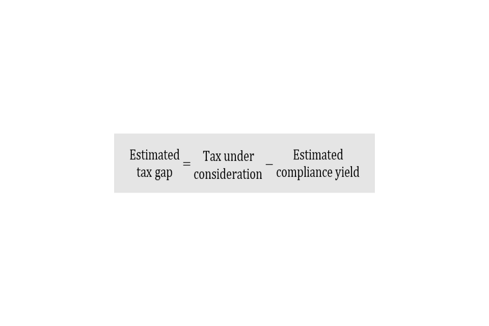
K8. The tax under consideration estimate relates to ongoing and completed enquiries. For completed enquiries, an estimate of tax under consideration is calculated from the compliance yield figures. This is calculated by applying the ratio of the compliance yield to tax under consideration from the taxpayer-level data to the actual compliance yield data.
K9. The compliance yield that is likely to be recovered for those under investigation is estimated using the ratio of the compliance yield to tax under consideration. This ratio is derived from the taxpayer-level data on completed avoidance enquiries.
Data quality
K10. The main source of error in these estimates is that HMRC may not identify all avoidance schemes – which will lead to an underestimation of the tax gap. It is difficult to quantify the extent to which this source of error impacts upon the estimates.
K11. There are a number of issues with the methodology to estimate the avoidance tax gap:
-
estimates of tax under consideration are made by tax specialists using all the information available at the time; as this information improves over time, the view of tax under consideration may change
-
the ratio of compliance yield to tax under consideration will change over time as more enquiries are completed; any difference between estimated compliance yield from ongoing enquiries and actual compliance yield will lead to revisions in the estimates
-
there is no tax year attached to the ‘tax under consideration’; therefore, the distribution of scheme uses and the scheme tax under consideration value across tax years are used to derive an annualised estimate
-
the scheme tax under consideration value is limited for the most recent tax year, therefore the estimate for 2020 to 2021 is a projection of the 2019 to 2020 estimate
-
Corporation Tax avoidance for large business groups is excluded from the calculations to avoid double-counting with the separate avoidance estimate for these businesses; any re-classification of users following more accurate information would lead to revisions of the Corporation Tax avoidance estimate
K12. As a result of these factors, the figures presented in the document are likely to be revised as more information becomes available.
K13. The data on avoidance schemes are reviewed by HMRC analysts for consistency and accuracy. Over time, as the scope, quality and quantity of the data improves, HMRC will seek to improve the avoidance tax gap estimates.
K14. In order to bring in more information about avoidance users, an additional step in methodology was introduced in ‘Measuring tax gaps 2021 edition’ to help redistribute the gap better across years. This brought in the scheme tax under consideration value alongside the number of usages.
Hidden economy
Moonlighters
K15. Moonlighters are defined as individuals who are employees in their legitimate occupation but do not declare earnings from other sources of income. There are 2 separate methodologies for different parts of the moonlighters estimate: one for earned income – that is individuals whose undeclared source of income is from employment – and one for unearned income – that is individuals whose undeclared source of income is not from employment but from sources such as lettings or interest.
K16. To calculate the earned income estimate, data from the Hidden Economy Quantitative Survey (HEQS) is used. The survey was commissioned by HMRC in 2015 to understand the nature of the hidden economy and the characteristics of those involved. Data on prevalence and income from hidden economy activities was captured as part of this research. In total, 9,640 respondents were surveyed.
K17. The estimate for unpaid tax on moonlighters’ earned income from the survey sample is calculated by subtracting the tax paid on declared income from the tax that would have been due on their earnings if they had declared all their income. This covers Income Tax and National Insurance contributions (NICs), with allowances made for whether the hidden economy activity in question would be classified as self-employment or employment. An allowance for under-reporting of income is also made in line with academic literature.
K18. This sample estimate is then grossed up to the total population by using the prevalence rates of moonlighters with earned income in the population. These prevalence rates are obtained from the HEQS and include weighting for non-response so that the prevalence rates are representative of the overall population.
K19. A time series for the moonlighters’ earned income estimate was created by using a proxy index which took into account changes in receipts over time as well as data from the Family Resources Survey. The Family Resources Survey is a government sponsored study which provides information about households in the UK. For more information on the Family Resources Survey go to GOV.UK.
K20. The tax gap for moonlighters’ unearned income covers those individuals who have additional sources of income that are not from employment. These sources of income would therefore require them to submit a Self Assessment return to supplement their normal tax payment through PAYE.
K21. The sources of income covered by unearned income are lettings, interest, capital gains on property, chargeable events, Individuals Savings Accounts (ISAs) and secondary income (for example, activities such as hobbies or online selling that are not regular enough to be considered employment).
K22. It is not necessary for most taxpayers to submit a Self Assessment return where all tax liabilities are withheld at source. For example, employment income where tax is deducted under PAYE, or basic rate tax withheld from bank interest. However, there are risks within this population, for example due to taxpayers not informing HMRC about sources of income, especially where they may exceed tax-free allowances. Where a Self Assessment return should have been completed, lettings, interest and ISA income would be subject to Income Tax; capital gains on property and chargeable events would be subject to Capital Gains Tax (CGT); and secondary income would be subject to Income Tax and NICs.
K23. HMRC cannot conduct random enquiries into the tax affairs of individuals who did not file a return because the legal position requires a return to be filed for an enquiry to take place. An alternative method is required for measurement of risks and estimating the associated tax gap.
K24. HMRC has therefore used data matching of administrative data and third-party information to measure the extent to which taxpayers fail to declare these additional sources of unearned income, with an estimate of additional tax due being calculated from the identified undeclared income. Third-party data matched with administrative tax records includes rental deposit schemes and bank and building society interest declarations. Because of the large amount of data involved in this exercise, data matching is only conducted on a representative sample of the population already in PAYE. The results are thereafter grossed up from the sample to produce an estimate of the overall tax gap from moonlighters’ unearned income.
K25. The limitations associated with the results of this exercise relate to the coverage of the third-party data used to establish evidence of additional undeclared income. Coverage varies across different sources of income, being especially good for lettings and interest income, whereas it is less reliable for the remaining sources identified. Additionally, there are other sources of income that could not be investigated due to unavailability of data. The resulting estimate should be interpreted broadly as a lower limit for the true scale of the tax gap relating to this group of taxpayers.
K26. The latest estimate of the tax gap relating to moonlighters’ unearned income is for tax year 2014 to 2015. This is projected forward based on receipts changes over time taking into account policy changes. For example, lettings income is subject to Income Tax; we take the lettings data-matching estimate for 2014 to 2015 and multiply it by a value which adds together Income Tax receipts for 2014 to 2015 and policy changes affecting receipts in 2015 to 2016 to obtain an estimate of how much policy changes have increased or decreased the Income Tax receipts.
K27. This approach allows the projections to take into account changes in both tax rates and the tax base over time. For example, increases in the personal allowance reduce the potential tax revenue from hidden economy activities, all else being equal. The projections are based on the Office for Budget Responsibility’s certified costings estimates for all Income Tax, NICs and CGT policy measures, and the relevant tax regime is applied for each of the unearned income sources.
K28. The projected figures for tax years 2017 to 2018 onwards are further adjusted to take into account the new “tax free allowance for landlords” that was introduced in April 2017.
Ghosts
K29. Ghosts are defined as individuals who do not declare any of their income to HMRC, be it earned or unearned.
K30. Data from the HEQS is used to estimate the ghosts tax gap. See the moonlighters section beginning at paragraph K16 for details.
K31. The estimate for unpaid tax on ghosts’ income from the survey sample is calculated by applying the relevant tax rate to the undeclared income estimated from the survey observations. This covers Income Tax and NICs, with allowances made for whether the hidden economy activity in question would be classified as self-employment or employment. An allowance for under-reporting of income is also made in line with academic literature.
K32. This sample estimate is then grossed up to the total population by using the prevalence rates of ghosts in the population. These prevalence rates are obtained from the HEQS and include weighting for non-response so that the prevalence rates are representative of the overall population.
K33. As with moonlighters, a time series for the ghosts tax gap estimate was created by using a proxy index which took into account changes in receipts over time as well as data from the Family Resources Survey.
K34. Like moonlighters, from tax year 2017 to 2018 onwards the figures are adjusted to reflect the impact of new “tax free allowance on self-employed traders” that was introduced in April 2017.